This is a reference and work in progress - I will continue adding to it as I come across more tools
Data wrangling is a crucial skill in data analysis. As you progress in your studies, you’ll encounter increasingly complex datasets that require sophisticated manipulation techniques. This section introduces you to some advanced tools that will expand your data wrangling toolkit.
Tip
To print the output of a command in R right away, you can enclose the code in parentheses (). This technique is often called “wrapping” or “enclosing” the expression. It is used throughout on this page.
Mastering Date-Time with lubridate
Dealing with dates and times can be tricky, but the lubridate package simplifies these tasks considerably. Let’s look at a practical example:
library(lubridate)# Converting string to date and extracting componentsdate_string<-"2023-10-12"(date_converted<-ymd(date_string))
Here, we’ve taken a date string, converted it to a date object, and then extracted its components. This is particularly useful when you’re working with time series data or need to analyze trends over time.
String Manipulation with stringr
The stringr package offers powerful tools for working with text data. Here’s how you might use it to extract information from a string:
library(stringr)# Example: Extracting, replacing, and counting string patterns(text<-"The deep blue ocean!")
These functions allow you to manipulate strings with ease, which is invaluable when cleaning text data or extracting specific information from larger text fields.
Joining Data with dplyr
When working with multiple datasets, you’ll often need to combine them. The dplyr package provides intuitive functions for this purpose:
# Left join(data_joined<-left_join(data_A, data_B, by ="id"))
  id var_A var_B
1  1     a  <NA>
2  2     b     d
3  3     c     e
This left join keeps all rows from data_A and adds matching information from data_B. It’s a common operation when you need to combine information from multiple sources while ensuring you don’t lose any records from your primary dataset.
Managing Categorical Data with forcats
The forcats package is designed to handle factor variables, which are crucial for representing categorical data in R:
# Lump levels(data_cat$species_lumped<-fct_lump(data_cat$species, n =2))
  [1] Other B     B     Other A     Other Other B     Other Other A     A
 [13] Other Other Other B     B     B     A     A     B     B     A     B
 [25] A     A     Other A     Other A     A     Other Other A     B     Other
 [37] A     B     B     Other Other Other Other B     Other Other Other Other
 [49] B     A     B     A     A     A     B     B     B     Other Other Other
 [61] B     Other A     Other A     Other Other A     Other Other B     A
 [73] A     Other B     B     B     A     B     B     Other Other B     B
 [85] Other B     Other A     Other Other A     Other Other Other B     Other
 [97] A     A     B     A
Levels: A B Other
  [1] C B B C A C C B C C A A C D D B B B A A B B A B A A D A D A A C D A B D A
 [38] B B C D D C B D D C C B A B A A A B B B D C D B D A D A C D A C C B A A D
 [75] B B B A B B C C B B C B D A C C A D C C B D A A B A
Levels: D A B C
Here, we’ve used fct_lump to combine less frequent categories into an “Other” group, and fct_relevel to manually reorder factor levels. These functions are useful when preparing categorical data for analysis or visualization.
Working with List-Columns using purrr
List-columns in data frames can be powerful but tricky to work with. The purrr package provides tools to handle these efficiently:
library(purrr)# Example: Applying a function to list column(nested_data<-tibble(x =1:3, y =list(1:3, 1:5, 1:10)))
# A tibble: 3 × 2
      x y
  <int> <list>
1     1 <int [3]>
2     2 <int [5]>
3     3 <int [10]>
# A tibble: 3 × 3
      x y          mean_y
  <int> <list>      <dbl>
1     1 <int [3]>     2
2     2 <int [5]>     3
3     3 <int [10]>    5.5
This example shows how to apply a function (in this case, mean) to each element of a list-column. It’s a powerful way to work with complex, nested data structures.
Efficient Large Dataset Handling with dtplyr
When working with large datasets, efficiency becomes crucial. The dtplyr package combines the speed of data.table with the syntax of dplyr:
Source: local data table [1 x 1]
Call:   `_DT1`[x > 0, .(mean_y = mean(y))]

     mean_y
      <dbl>
1 0.0000310

# Use as.data.table()/as.data.frame()/as_tibble() to access results
This approach allows you to work with large datasets more efficiently, using familiar dplyr syntax.
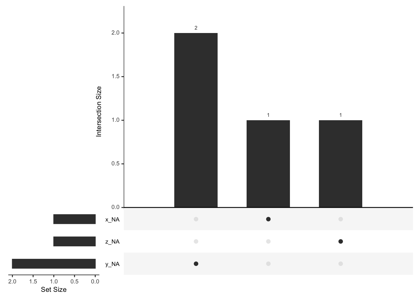
Handling Missing Data with naniar
The naniar package provides sophisticated tools for exploring and handling missing data.
library(naniar)# Create sample data with missing valuesdf<-data.frame( x =c(1, 2, NA, 4, 5), y =c(NA, 2, 3, NA, 5), z =c(1, NA, 3, 4, 5))# Visualize missing data patternsgg_miss_upset(df)
# Calculate the percentage of missing datapct_miss(df)
  x        y    z
1 1 3.333333 1.00
2 2 2.000000 3.25
3 3 3.000000 3.00
4 4 3.333333 4.00
5 5 5.000000 5.00
Understanding and properly handling missing data is crucial for maintaining the integrity of your analyses.
Text Mining with tidytext
The tidytext package allows you to perform text mining tasks within the tidyverse framework.
library(tidytext)library(dplyr)# Sample text datatext_data<-tibble( line =1:3, text =c("The quick brown fox","jumps over the lazy dog","The dog was not amused"))# Tokenize the texttokens<-text_data%>%unnest_tokens(word, text)# Count word frequenciesword_frequencies<-tokens%>%count(word, sort =TRUE)print(word_frequencies)
# A tibble: 11 × 2
   word       n
   <chr>  <int>
 1 the        3
 2 dog        2
 3 amused     1
 4 brown      1
 5 fox        1
 6 jumps      1
 7 lazy       1
 8 not        1
 9 over       1
10 quick      1
11 was        1
This approach is valuable for analyzing large text datasets, sentiment analysis, or preparing text data for machine learning models.