In many research scenarios, we’re interested in how things change over time or under different conditions. Repeated measures ANOVA is a powerful tool for these situations. It’s particularly useful when we measure the same subjects multiple times, like tracking an individual’s performance across different time points or conditions.
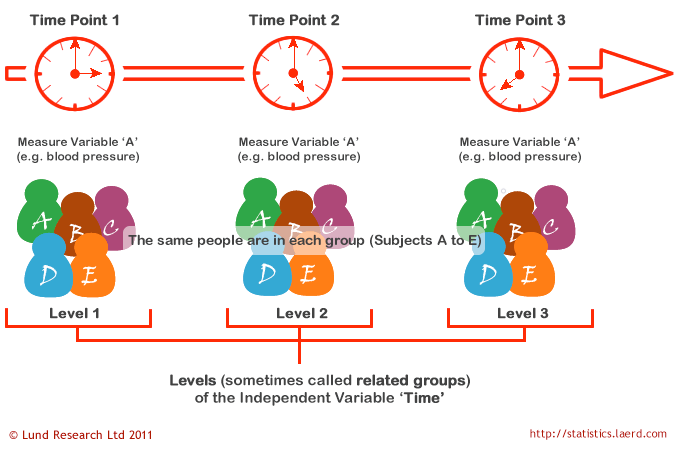
Repeated Measures Design
The key feature of repeated measures designs is that they account for the correlation between measurements taken on the same subject. This correlation is important because an individual’s responses are often more similar to their own previous responses than to those of other individuals.
The Null Hypothesis in Repeated Measures ANOVA
In repeated measures ANOVA, we often have two types of effects: between-subjects effects and within-subjects effects. The between-subjects effects compare different groups of subjects, while the within-subjects effects examine changes within the same subjects over time or conditions.
The null hypothesis for between-subjects effects is that the mean response remains consistent across different groups, while for within-subjects effects, the null hypothesis is that the mean response remains consistent across repeated measurements.
A Real-World Example: Sea Lion Pulse Rates
Let’s look at a practical example to see how repeated measures ANOVA works. We’ll examine data from a study on sea lions, where researchers measured pulse rates under different conditions.
exertype: Type of activity (1 = rest, 2 = walking, 3 = swimming)
pulse: Measured pulse rate
time: Time point of measurement (1, 2, or 3)
Note the use of factors, which are essential for repeated measures ANOVA to work correctly. Factors here represent categorical variables, like diet type or activity. Factors have order, which is important for interpreting the results.
Visualizing the Data
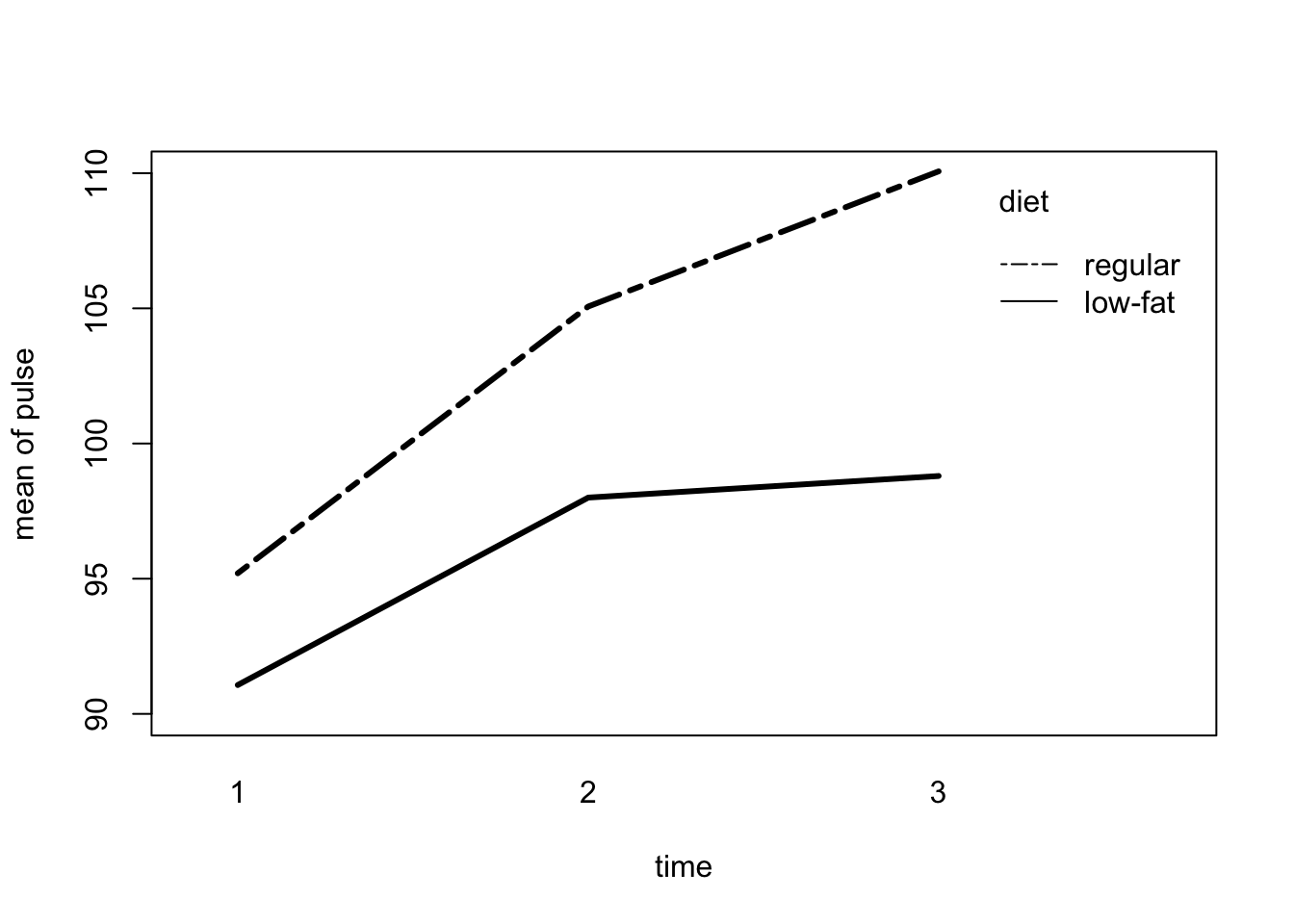
Before the analysis, let’s visualize our data to get a sense of what’s happening:
This plot shows how pulse rates change over time for each diet group. We can see that both groups show an increase in pulse rate over time, but the rate of increase appears different between the two diets, with low fat diet group being associated with lower mean pulse.
Performing Repeated Measures ANOVA
Now, let’s run our repeated measures ANOVA:
diet.aov<-aov(pulse~diet*time+Error(id), data =sealion)summary(diet.aov)
Error: id
          Df Sum Sq Mean Sq F value Pr(>F)
diet       1   1262    1262   3.147 0.0869 .
Residuals 28  11227     401
---
Signif. codes:  0 '***' 0.001 '**' 0.01 '*' 0.05 '.' 0.1 ' ' 1

Error: Within
          Df Sum Sq Mean Sq F value   Pr(>F)
time       2   2067  1033.3  11.808 5.26e-05 ***
diet:time  2    193    96.4   1.102    0.339
Residuals 56   4901    87.5
---
Signif. codes:  0 '***' 0.001 '**' 0.01 '*' 0.05 '.' 0.1 ' ' 1
Let’s break down this output:
Error: id: This part shows the between-subjects effects. Here, we see a marginally significant effect of diet (p = 0.0869).
Error: Within: This shows the within-subjects effects. We see a highly significant effect of time (p = 5.26e-05), but no significant interaction between diet and time (p = 0.339).
What does this tell us? Pulse rates change significantly over time, regardless of diet. The effect of diet itself is borderline significant, suggesting a possible overall difference between diet groups. However, the lack of a significant interaction indicates that the pattern of change over time is similar for both diet groups.
Exploring Different Factors: Exercise Type
Let’s also look at how exercise type affects pulse rates:
exertype.aov<-aov(pulse~exertype*time+Error(id), data =sealion)summary(exertype.aov)
Error: id
          Df Sum Sq Mean Sq F value   Pr(>F)
exertype   2   8326    4163      27 3.62e-07 ***
Residuals 27   4163     154
---
Signif. codes:  0 '***' 0.001 '**' 0.01 '*' 0.05 '.' 0.1 ' ' 1

Error: Within
              Df Sum Sq Mean Sq F value   Pr(>F)
time           2   2067  1033.3   23.54 4.45e-08 ***
exertype:time  4   2723   680.8   15.51 1.65e-08 ***
Residuals     54   2370    43.9
---
Signif. codes:  0 '***' 0.001 '**' 0.01 '*' 0.05 '.' 0.1 ' ' 1
This analysis shows:
Error: id shows the between-subjects effects. The significant effect of exercise type (p = 3.62e-07) indicates that overall pulse rates differ among the exercise types (rest, walking, swimming), regardless of time.
Error: Within shows the within-subjects effects:
The significant effect of time (p = 4.45e-08) means pulse rates change over the three time points, regardless of exercise type.
The significant interaction between exercise type and time (p = 1.65e-08) suggests that how pulse rates change over time depends on the exercise type.
In simpler terms:
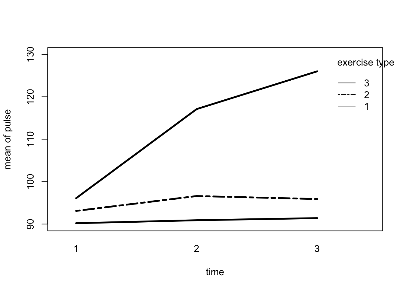
Different exercises lead to different pulse rates.
Pulse rates change as time passes.
The way pulse rates change over time is not the same for all exercise types.
For example, pulse rates might increase more rapidly over time during swimming compared to walking, or they might plateau quickly during rest but continue rising during active exercises.
Interpreting the Results
Taken together, these analyses paint a comprehensive picture of how sea lion pulse rates are affected by various factors:
Time consistently shows a significant effect, indicating that pulse rates change over the course of the experiment, regardless of other factors.
Diet shows a non-significant effect, but it is close to 0.05, hinting at possible overall differences between diet groups, but more sampling may be needed to detect a significant effect, should there be one.
Exercise type has a strong effect on pulse rates and significantly influences how those rates change over time.
This example illustrates the power of repeated measures ANOVA in teasing apart complex relationships in data where we have multiple measurements from the same subjects. By accounting for individual differences (through the Error(id) term), we can more accurately assess the effects of our experimental variables.
Remember, repeated measures designs are particularly valuable when individual differences are large, as they allow us to control for these differences and focus on the effects of our experimental manipulations.
Further Reading
This page contains a surface-level introduction to repeated measures, for more in depth understanding of assumptions, theory, consult these sources :