Multivariate Data Analysis

A correlation heatmap from an ongoing analysis I am working on

Introduction to Multivariate Data

Multivariate data sets involve multiple response variables recorded from each sampling unit. These data structures allow for the examination of complex relationships between variables, providing a more comprehensive understanding of the system under study. In statistical analysis, multivariate methods are crucial for exploring, describing, and modeling the interdependencies among variables.

Let’s generate a multivariate dataset to illustrate these concepts:

library(tibble)
library(ggplot2)

set.seed(456)  # For reproducibility

multivariate_data <- tibble(
  protein_content = rnorm(100, mean = 20, sd = 5),
  hours_of_activity = rnorm(100, mean = 5, sd = 2),
  weight = 70 + 0.5 * protein_content - 2 * hours_of_activity + rnorm(100, mean = 0, sd = 5),
  blood_pressure = 120 + 0.2 * protein_content - 1.5 * hours_of_activity + rnorm(100, mean = 0, sd = 10)
)

In this dataset, we explore the effects of dietary protein content and physical activity levels on weight and blood pressure in a simulated population. Multiple variables are recorded for each individual, allowing us to investigate the relationships between these factors.

Correlation Analysis in Multivariate Data

A fundamental approach to understanding multivariate relationships is through correlation analysis. The correlation matrix provides a comprehensive view of pairwise relationships between variables. For a dataset with p variables, the correlation matrix is a p × p symmetric matrix where each element r_ij represents the correlation coefficient between variables i and j.

Let’s compute and examine the correlation matrix for our dataset:

cor_matrix <- cor(multivariate_data)
print(cor_matrix)

                  protein_content hours_of_activity     weight blood_pressure
protein_content        1.00000000       -0.01704504  0.4637094     0.09399024
hours_of_activity     -0.01704504        1.00000000 -0.5594361    -0.24380084
weight                 0.46370939       -0.55943611  1.0000000     0.15118056
blood_pressure         0.09399024       -0.24380084  0.1511806     1.00000000

The correlation coefficients range from -1 to 1, where -1 indicates a perfect negative linear relationship, 1 indicates a perfect positive linear relationship, and 0 suggests no linear relationship.

To visualize these relationships more intuitively, we can create a correlation heatmap:

library(reshape2)  # for melt function, this can also be completed with pivot_longer

rownames(cor_matrix) <- colnames(cor_matrix) <- c("protein_content", "hours_of_activity", "weight", "blood_pressure")
melted_cor_matrix <- melt(cor_matrix)

ggplot(data = melted_cor_matrix, aes(x=Var1, y=Var2)) +
  geom_tile(aes(fill=value), color='white') +
  geom_text(aes(label=sprintf("%.2f", value)), vjust=1) +
  scale_fill_gradient2(low="blue", high="red", mid="white", midpoint=0, limit=c(-1,1), name="Correlation") +
  theme_minimal() + 
  theme(axis.text.x = element_text(angle=45, vjust=1, size=12, hjust=1)) +
  coord_fixed()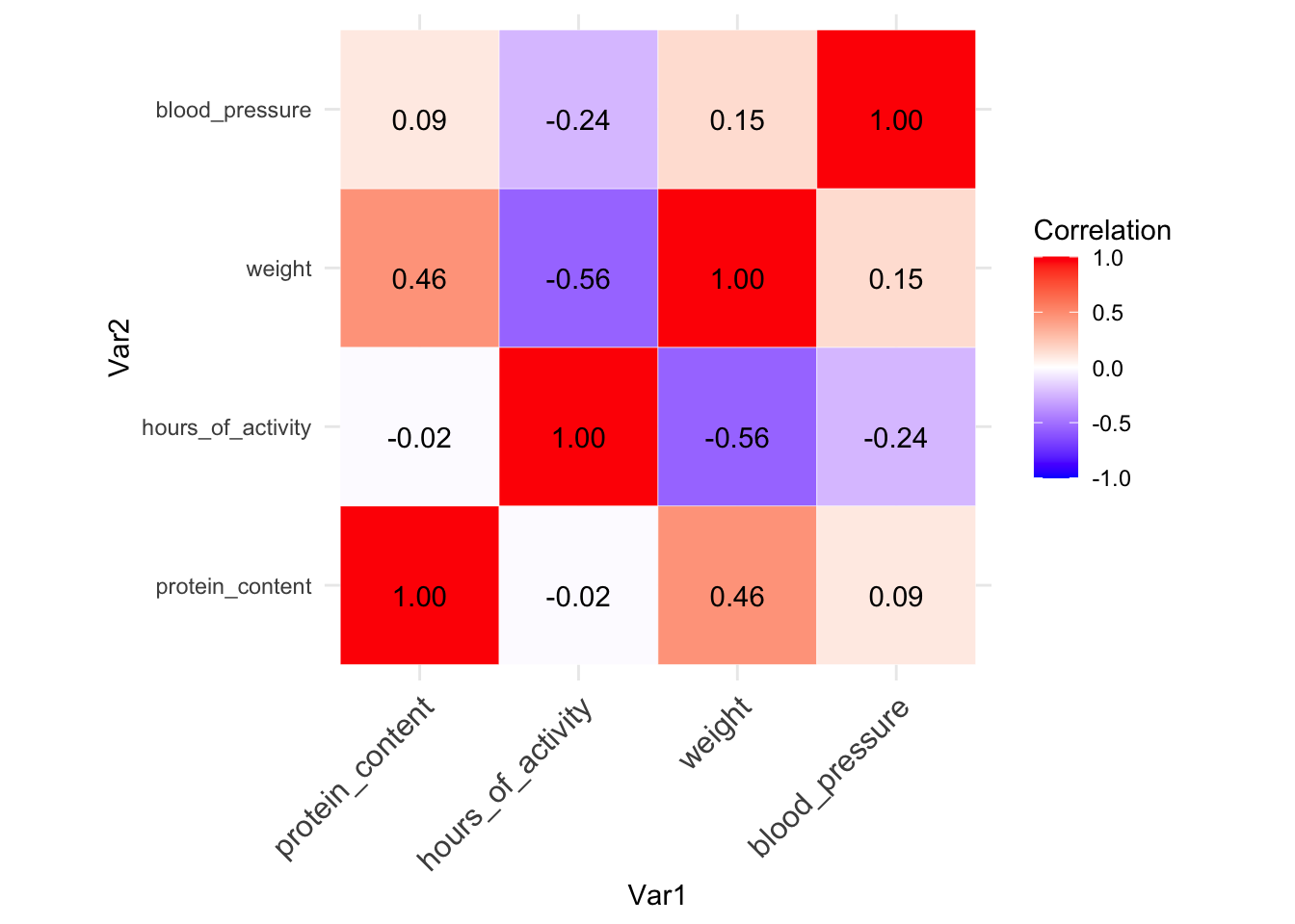

Interpreting Multivariate Correlations

The correlation matrix and heatmap reveal several key relationships in our data:

The correlation between protein_content and hours_of_activity is near zero (-0.02), indicating no significant linear relationship between these variables. This suggests that in our simulated population, dietary protein intake is not associated with physical activity levels.

Protein_content shows a moderate positive correlation (0.46) with weight. This positive relationship indicates that higher protein intake is associated with higher weight in our dataset. However, it’s crucial to note that correlation does not imply causation, and other factors may influence this relationship.

Hours_of_activity demonstrates a stronger negative correlation (-0.56) with weight. This inverse relationship aligns with the expectation that increased physical activity is associated with lower weight.

Blood_pressure exhibits weak correlations with protein_content (0.09) and weight (0.15), but a stronger negative correlation (-0.24) with hours_of_activity. This suggests that among our variables, physical activity might have the most substantial association with blood pressure.

Advanced Multivariate Techniques

While correlation analysis provides valuable insights, more advanced techniques can further elucidate the structure of multivariate data:

Principal Component Analysis (PCA) is a dimension reduction technique that identifies orthogonal axes (principal components) that capture the maximum variance in the data. PCA can reveal underlying patterns and reduce the dimensionality of complex datasets.

Multivariate Regression extends simple linear regression to multiple dependent variables. It allows for the simultaneous modeling of multiple response variables as functions of predictor variables.

Canonical Correlation Analysis (CCA) examines the relationships between two sets of variables, finding linear combinations of variables in each set that are maximally correlated with each other.