Pivot Tables – Research Methods Lab

Utility of Pivot Tables

Pivot tables offer several key advantages in data analysis:

Data Summarization Transform extensive datasets into meaningful tables, charts, or reports, facilitating trend identification and data point comparison.
Dynamic Analysis The drag-and-drop functionality allows for rapid changes in data layout and view, enabling analysis from multiple perspectives.
Segmented Views Break down large datasets by categories such as regions, products, or time periods, enhancing data digestibility.

Creating a Pivot Table

Follow these steps to create a pivot table:

Select the Dataset Highlight the range of cells containing your data.
Navigate to Insert Tab Click on the ‘Insert’ tab in Excel’s ribbon, then choose ‘PivotTable’.
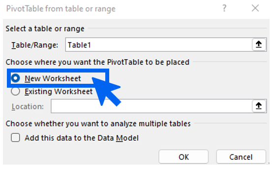
Choose Data Range and Location In the dialog box, specify the data range and where to place the Pivot Table. Typically, select the entire dataset and place the Pivot Table in a new worksheet.
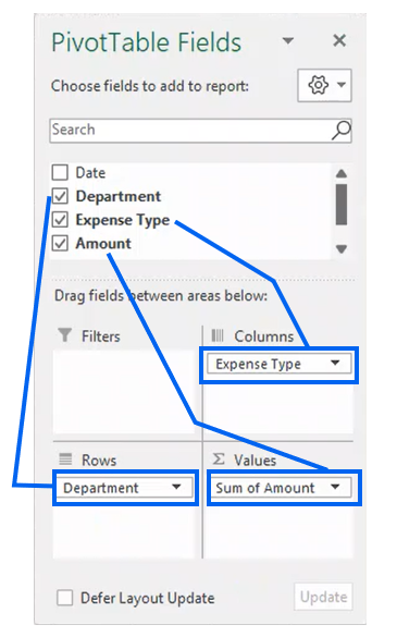
Organize Data Using Field List Once the blank Pivot Table is created, use the “PivotTable Field List” pane to drag and drop fields into the Rows, Columns, Values, and Filters areas.
Analyze and Customize Refine and customize your table, convert to tabular format, or copy and paste for secondary formula application.

Excel Pivot Table Best Practices

Data Preparation Ensure your data is clean, organized, and free of blank rows or columns before creating a pivot table.
Source Data Awareness Remember to refresh the pivot table after modifying the original data (adding, removing, or modifying rows/columns).
Report Filters Use report filters to analyze data subsets without altering the entire table.
Field Arrangement Experiment with dragging and dropping fields between rows, columns, values, and filters to find the most insightful data view.

Pivot Table Formatting

Changing to Tabular Format

Click anywhere in the pivot table to display the PivotTable Tools on the ribbon.
Go to the Design tab.
To remove subtotals, click on the Subtotals dropdown and select Don't Show Subtotals.
To remove grand totals, click on the Grand Totals dropdown and select Off for Rows and Columns.
In the Report Layout dropdown, select Show in Tabular Form.
To repeat item labels, go back to the Report Layout dropdown and select Repeat All Item Labels.

Displaying Items with No Data

Right-click an item in the pivot table field, and in the pop-up menu, click Field Settings.
In the Field Settings dialog box, click the Layout & Print tab.
In the Layout section, check the box for ‘Show items with no data’.

Replacing Missing Values with Zero

Right-click on any cell within the pivot table.
Select PivotTable Options.
In the Layout & Format tab, check the For empty cells show option and enter 0 in the adjacent box.
Click OK.

Applying Formulae on Pivot Table Data

When performing calculations on summarized pivot table data, it’s advisable to copy the pivot table and paste as values elsewhere on the sheet. This approach is preferable because clicking on a cell in the pivot table executes a GetPivotData function, which is less straightforward than a simple cell cross-reference (e.g., =C4).

R Implementation

While Excel is commonly used for pivot tables, R offers similar functionality through packages like dplyr and tidyr. Here’s an example of how to create a pivot table-like summary in R:

library(dplyr)
library(tidyr)

# Sample data
data <- data.frame(
  Date = as.Date('2023-01-01') + 0:364,
  Product = sample(c("A", "B", "C"), 365, replace = TRUE),
  Sales = runif(365, 100, 1000)
)

# Creating a pivot table-like summary
pivot_summary <- data %>%
  mutate(Month = format(Date, "%Y-%m")) %>%
  group_by(Month, Product) %>%
  summarise(Total_Sales = sum(Sales)) %>%
  spread(Product, Total_Sales)

print(pivot_summary)

# A tibble: 12 × 4
# Groups:   Month [12]
   Month       A     B     C
   <chr>   <dbl> <dbl> <dbl>
 1 2023-01 2491. 8304. 5290.
 2 2023-02 5752. 6680. 4337.
 3 2023-03 7200. 4195. 5592.
 4 2023-04 7884. 5148. 4259.
 5 2023-05 5005. 8508. 5196.
 6 2023-06 5804. 5240. 5448.
 7 2023-07 3989. 7217. 6369.
 8 2023-08 9584. 1961. 6605.
 9 2023-09 2241. 6921. 7751.
10 2023-10 4298. 4165. 6377.
11 2023-11 5050. 5828. 3590.
12 2023-12 8612. 4958. 5561.

This R code creates a summary similar to an Excel pivot table, grouping sales by month and product.

Test Your Understanding

Let’s test your understanding of pivot tables with a quick quiz: