Conducting T-Tests in R the Long Way

Consider this example data…

Background: Ocean acidification is a result of increased carbon dioxide (CO₂) in the atmosphere. As more CO₂ is absorbed by the ocean, it reacts with seawater to produce carbonic acid, which subsequently lowers the ocean’s pH. This can affect marine life, especially shellfish and corals, which rely on carbonate ions to build their shells and skeletons.

Scientific Hypothesis: Ocean acidification significantly affects the growth of shellfish.

Data Collection: Researchers collect a sample of shellfish and divide them into two groups. One group (Control) is kept in seawater with a pH close to current levels. The other group (Treated) is kept in seawater with a lower pH, simulating future predicted levels of ocean acidification.

After a specified period, the growth (e.g., increase in shell length) of the shellfish in each group is measured.

Sample Data:

Control Group (current pH level): Growth in mm: [2.1, 2.3, 2.2, 2.4, 2.5, 2.3, 2.4, 2.2, 2.3, 2.1]
Treated Group (lower pH level): Growth in mm: [1.8, 1.9, 1.7, 1.9, 1.8, 1.7, 1.9, 1.8, 1.7, 1.8]

The researchers want to know if the difference in growth between the two groups is statistically significant.

Performing a t-test by hand involves several steps. Below are the steps to perform an independent two-sample t-test by hand along with the corresponding R code:

# Sample data
dat <- data.frame(
  control = c(2.1, 2.3, 2.2, 2.4, 2.5, 2.3, 2.4, 2.2, 2.3, 2.1),
  treated = c(1.8, 1.9, 1.7, 1.9, 1.8, 1.7, 1.9, 1.8, 1.7, 1.8)
)

head(dat)

  control treated
1     2.1     1.8
2     2.3     1.9
3     2.2     1.7
4     2.4     1.9
5     2.5     1.8
6     2.3     1.7

# remember tabular data have one observation per row and one variable per column.
# these data are NOT in tabular form. 

# 1. data# 1. Calculate the sample means
mean_control <- mean(dat$control)
mean_treated <- mean(dat$treated)

# 2. Calculate the sample variances
var_control <- var(dat$control)
var_treated <- var(dat$treated)

# 3. Calculate the pooled variance
n1 <- length(dat$control)
n2 <- length(dat$treated)

pooled_var <- ((n1 - 1) * var_control + (n2 - 1) * var_treated) / (n1 + n2 - 2)

# 4. Calculate the t-statistic
t_statistic <- (mean_control - mean_treated) / sqrt(pooled_var * (1/n1 + 1/n2))

# 5. Determine the degrees of freedom
df <- n1 + n2 - 2

# 6. Compare the calculated t-statistic to the critical t-value
alpha <- 0.05
critical_value <- qt(1 - alpha/2, df)  # For a two-tailed test
significant <- abs(t_statistic) > critical_value

# Calculate the p-value
if (t_statistic > 0) {
    p_value <- 2 * (1 - pt(t_statistic, df))
} else {
    p_value <- 2 * pt(t_statistic, df)
}

# Results
results <- list(mean_control = mean_control, mean_treated = mean_treated, 
                t_statistic = t_statistic, df = df, pvalue = p_value, significant = significant)

results

$mean_control
[1] 2.28

$mean_treated
[1] 1.8

$t_statistic
[1] 9.797959

$df
[1] 18

$pvalue
[1] 1.22155e-08

$significant
[1] TRUE

Tip

if you want to print any small number as a number instead of in scientific notation, run this. scipen is the number of significant digits to print in scientific notation. Setting it to a large number will prevent R from printing numbers in scientific notation.

options(scipen=1000000000)

The p value is 0.00000001, which is much less than 0.05, so we can reject the null hypothesis that the two groups have the same growth rate.

Lets plot!

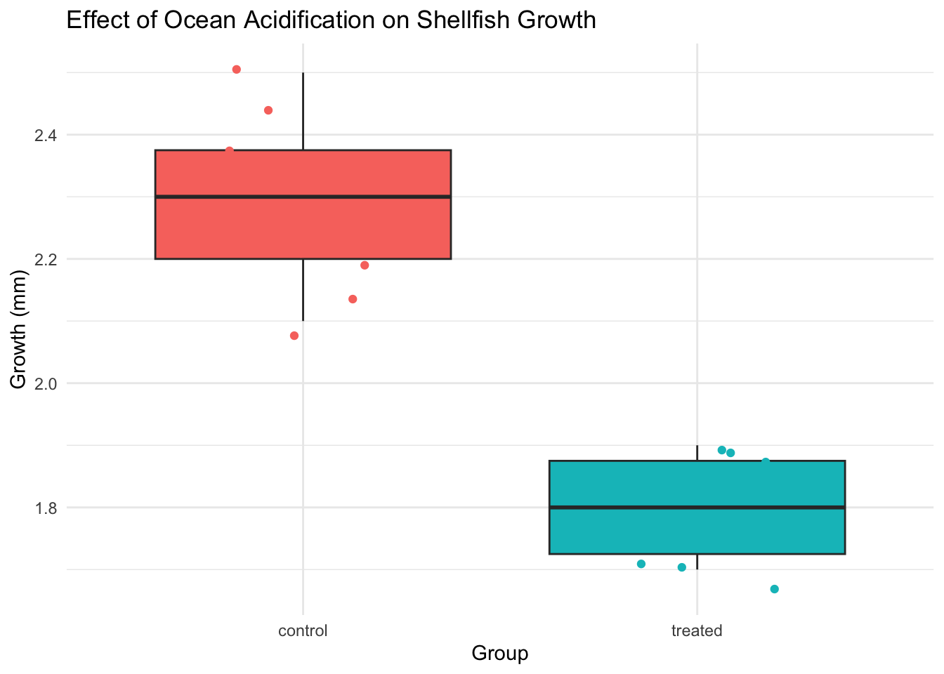
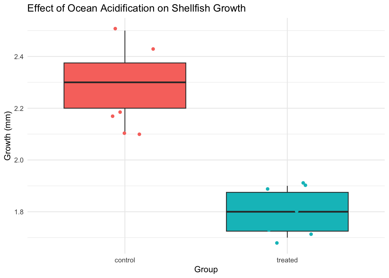
# Required library
library(tidyverse)
library(ggplot2)

# Prepare data for plotting
# here we are making it long by pivoting longer, so that we have a new column indicating our grouping variable and another indicating the measured variable (Growth)
datlong <- dat %>% 
  pivot_longer(cols = c(control, treated), names_to = "Group", values_to = "Growth")

# Create the plot
ggplot(datlong, aes(x=Group, y=Growth)) +
  geom_boxplot(aes(fill=Group)) +
  geom_jitter(width=0.2, aes(color=Group)) +
  labs(title="Effect of Ocean Acidification on Shellfish Growth",
       y="Growth (mm)") +
  theme_minimal()+ 
  theme(legend.position = "NONE")

p <- ggplot(datlong, aes(x=Group, y=Growth)) +
  geom_boxplot(aes(fill=Group)) +
  geom_jitter(width=0.2, aes(color=Group)) +
  labs(title="Effect of Ocean Acidification on Shellfish Growth",
       y="Growth (mm)") +
  theme_minimal()+ 
  theme(legend.position = "NONE")

p

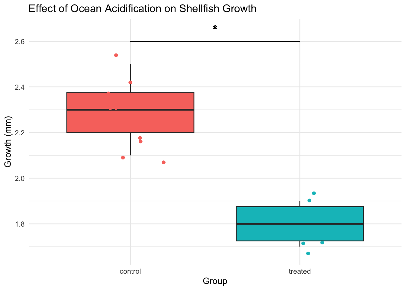
# If p-value is less than 0.05, add a significance indicator
if (p_value < 0.05) {
  p <- p + 
    geom_segment(aes(x = 1, xend = 2, y = max(Growth) + 0.1, yend = max(Growth) + 0.1)) + 
    geom_text(aes(x = 1.5, y = max(Growth) + 0.15, label = "*"), size = 6)
}

p

now, that was a lot of work to get that significance though, though wasn’t it?

spoiler alert: we can use t.test()

t.test(Growth ~ Group, datlong, var.equal = TRUE)


    Two Sample t-test

data:  Growth by Group
t = 9.798, df = 18, p-value = 0.00000001222
alternative hypothesis: true difference in means between group control and group treated is not equal to 0
95 percent confidence interval:
 0.3770763 0.5829237
sample estimates:
mean in group control mean in group treated 
                 2.28                  1.80