Chi-square Test of Independence

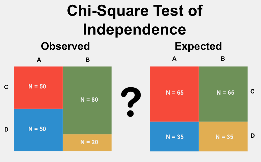
While the mathematics mirrors goodness-of-fit testing, independence tests calculate expected frequencies differently. Instead of using theoretical expectations, we derive expected frequencies from the observed data itself. This approach helps us understand relationships between categorical variables.

The core question in independence testing is whether two categorical variables influence each other. For example, does education level affect voting patterns? Or does genetic variation relate to disease risk? We express this formally through our null hypothesis (\(H_0\)): the proportions of one variable remain constant across different levels of the second variable.

Real-World Applications

Let’s examine two compelling examples that show how independence testing works in practice.

Safety Equipment and Injury Patterns

A study of bicycle accidents in New South Wales examined the relationship between helmet use and injury type. This straightforward 2×2 analysis carries important public health implications:

Input = ("
PSE        Head.injury  Other.injury
Helemt     372          4715
No.helmet  267          1391
")

Matriz = as.matrix(read.table(
  textConnection(Input),
  header = TRUE,
  row.names = 1
))

# View the data
Matriz

          Head.injury Other.injury
Helemt            372         4715
No.helmet         267         1391

# Test with continuity correction
chisq.test(Matriz, correct = TRUE)


    Pearson's Chi-squared test with Yates' continuity correction

data:  Matriz
X-squared = 111.66, df = 1, p-value < 2.2e-16

# Test without correction (if > 2x2 ) 
chisq.test(Matriz, correct = FALSE)


    Pearson's Chi-squared test

data:  Matriz
X-squared = 112.68, df = 1, p-value < 2.2e-16

The remarkably small p-value (3×10⁻²⁶) reveals a clear pattern: cyclists without helmets suffer proportionally more head injuries. The continuation correction, appropriate for 2×2 tables, ensures our conclusion is conservative and robust.

Note

In the chisq.test() function in R, the correct parameter determines whether Yates’ continuity correction is applied to the chi-squared test for a 2x2 table:

correct = TRUE: This applies Yates’ continuity correction. This correction is used to make the chi-squared test more accurate for small sample sizes, specifically for 2x2 contingency tables. It slightly reduces the chi-squared value to adjust for the fact that the test may be overly sensitive with small datasets. The correction helps reduce Type I errors (false positives) but might be conservative.
correct = FALSE: This disables the continuity correction, which means that the chi-squared test is performed in its standard form without any adjustment. This is typically used when you have a larger sample size or if you don’t need the conservative nature of the corrected test.

Genetics and Disease Risk

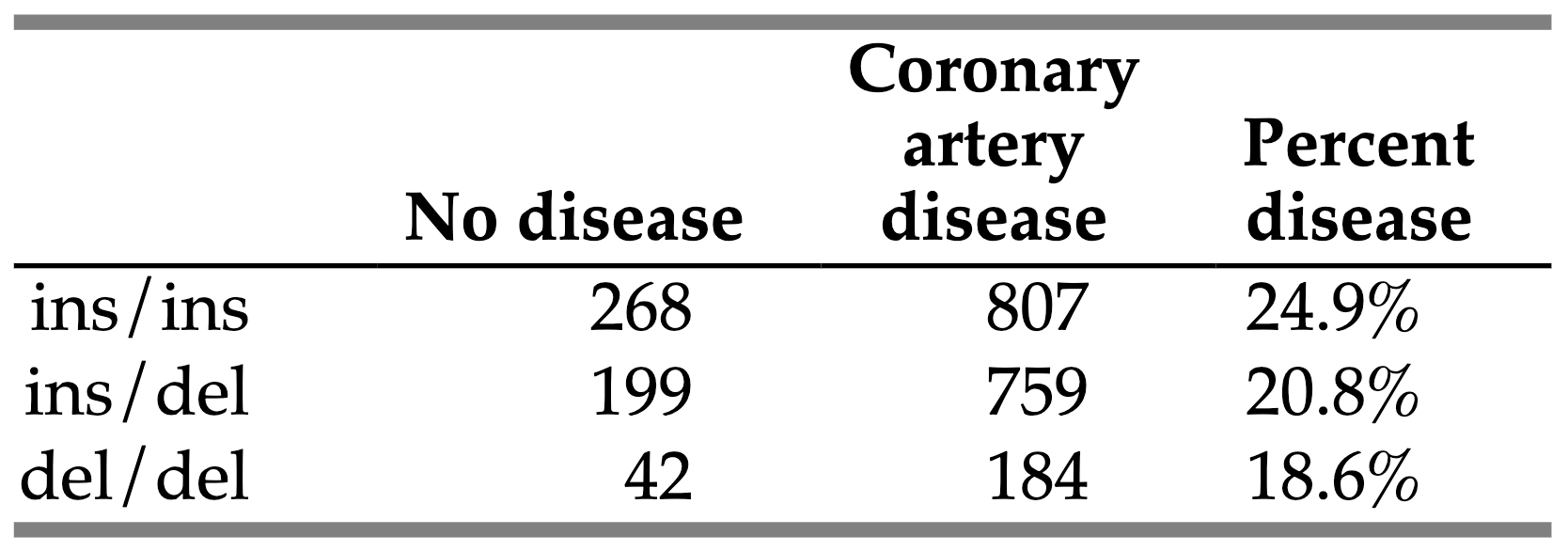
A more complex example comes from genetic epidemiology. Researchers studied how variations in the apolipoprotein B gene might influence heart disease risk. They examined three genetic variants (ins/ins, ins/del, del/del) against disease status:

Input =("
Genotype  Health       Count
ins-ins   no_disease   268
ins-ins   disease      807
ins-del   no_disease   199
ins-del   disease      759
del-del   no_disease    42
del-del   disease      184
")

Data.frame = read.table(textConnection(Input),header=TRUE)

# Create and view the contingency table
Data.xtabs = xtabs(Count ~ Genotype + Health,
                   data=Data.frame)

Data.xtabs

         Health
Genotype  disease no_disease
  del-del     184         42
  ins-del     759        199
  ins-ins     807        268

summary(Data.xtabs)

Call: xtabs(formula = Count ~ Genotype + Health, data = Data.frame)
Number of cases in table: 2259 
Number of factors: 2 
Test for independence of all factors:
    Chisq = 7.259, df = 2, p-value = 0.02652

# Run the independence test     
chisq.test(Data.xtabs)


    Pearson's Chi-squared test

data:  Data.xtabs
X-squared = 7.2594, df = 2, p-value = 0.02652

The chi-square value of 7.26 (p=0.027) suggests genetic variation does influence disease risk. Unlike our helmet example, this analysis used three categories, giving us two degrees of freedom. The relationship here is subtler but still statistically significant.

When interpreting independence tests, remember that statistical significance doesn’t always mean practical importance. Consider your sample size, study design, and real-world implications alongside the p-value. For small samples or low expected frequencies, Fisher’s Exact Test might provide a more reliable alternative.