data_fish_mpa <- read.csv("https://raw.githubusercontent.com/laurenkolinger/MES503data/main/week7/fish_biomass_mpa.csv")Introduction to ANOVA
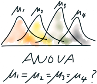
Analysis of Variance, commonly known as ANOVA, is a powerful statistical technique that extends our ability to analyze relationships between variables. While t-tests allow us to compare means between two groups, ANOVA enables us to examine differences among multiple groups simultaneously.
The Purpose of ANOVA
Imagine you’re investigating how different environmental factors affect a specific outcome. With ANOVA, you can address questions like: “Do different habitat types significantly influence species diversity?” This technique is particularly valuable when you have:
- One continuous dependent variable (e.g., species diversity)
- One or more categorical independent variables (e.g., habitat types)
ANOVA’s primary goal is to determine whether there are statistically significant differences between the means of three or more independent groups.
Why Not Multiple T-tests?
We previously learned a technique for comparing the means of two groups, the t-test. You might wonder why we don’t simply conduct multiple t-tests to compare groups.
The key issue here is conducting multiples of any statistical test increases the risk of Type I errors. Each time you perform a statistical test, there’s a chance of falsely rejecting the null hypothesis (i.e., finding a significant difference when there isn’t one). As you increase the number of comparisons, this risk compounds.
ANOVA solves this problem by analyzing all groups simultaneously, maintaining the overall error rate at your chosen significance level (typically 0.05).
ANOVA Assumptions
For ANOVA results to be reliable and valid, certain assumptions must be met:
Independence: Each data point should be independent of others. In practical terms, this means that the value of one observation shouldn’t influence or be influenced by another observation.
Normality: The residuals (differences between observed and predicted values) should follow a normal distribution. This assumption ensures that the variability in your data is random and not systematically skewed.
Homogeneity of Variances: The variance within each group should be approximately equal. This assumption, also known as homoscedasticity, ensures that one group’s variance isn’t significantly different from another’s.
These assumptions are crucial because they underpin the mathematical framework of ANOVA. Violating these assumptions can lead to unreliable results and incorrect conclusions.
Note
Look familiar? These assumptions are the same for t-tests and linear regression.
Types of ANOVA
ANOVA is a flexible technique that can be applied in various research scenarios:
One-way ANOVA: This is the simplest form, used when you have one independent variable with three or more levels or groups. It tests if there are any statistically significant differences between the means of these groups.
Two-way ANOVA: This method is employed when you have two independent variables. It not only looks at the individual impact of each variable but also if there’s a combined effect (interaction) between them.
Multi-way ANOVA: Used when there are more than two independent variables. It’s a generalized form that can test the effect of multiple factors simultaneously.
This week we are only focusing on one-way ANOVA, and in the next week we will be getting into these other types of ANOVA. Just be aware that ANOVA is much more than looking at one response across 3 or more levels of a grouping variable.
ANOVA terms
Lets introduce some basic terminology :
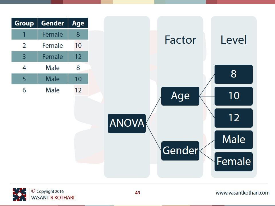
- Factors: These are the independent variables in your experiment. Factors are the conditions or characteristics you manipulate or observe to study their effect on the outcome.
Levels: Each factor has different categories or values, which are called levels. For example, if “treatment” is a factor, its levels might be “control,” “low dose,” and “high dose”.
Main Effect: The direct influence of a single factor on the response variable, independent of other factors (this will become more clear as we get introduced to other effect types, such as interaction effects, and random effects)
Example Dataset: Fish Biomass in Marine Protected Areas (MPAs)
To illustrate ANOVA, let’s consider a dataset from a study on marine conservation:
Background: Researchers are investigating if different types of Marine Protected Areas (MPAs) have varying effects on fish biomass. They’ve categorized MPAs into three types:
- No-Take: These are pristine zones where no fishing is allowed, acting as refuges for marine life.
- Limited-Take: Fishing is permissible here but under strict regulations. There may be restrictions on fishing methods, species, or quantity.
- Open Access: Fishing is allowed with minimal oversight.
Goal of the study: Understand if fish biomass (measured in kg) is influenced by the type of MPA.
Let’s import the data and take a look at the first few rows:
| MPA_Type | Fish_Biomass |
|---|---|
| notake | 104.96714 |
| notake | 98.61736 |
| notake | 106.47689 |
| notake | 115.23030 |
| notake | 97.65847 |
| notake | 97.65863 |
Dataset Description
Rows: Each entry represents a sample from a specific MPA type. There are 150 samples in total, evenly distributed among the three MPA types.
-
Columns:
- MPA_Type: Specifies the MPA category for the sample (No-Take, Limited-Take, or Open Access).
- Fish_Biomass: Indicates the biomass of fish observed in that sample, given as a continuous value in kg.
Hypotheses in ANOVA
In ANOVA, we formulate and test specific hypotheses:
- Null Hypothesis (\(H_0\)): There is no difference among group means.
- Alternative Hypothesis (\(H_a\)): At least one group mean differs from the others.
For our fish biomass study:
- \(H_0\): There is no difference in average fish biomass across all MPA types.
- \(H_a\): The average fish biomass varies for at least one MPA type.