# ========================================# Data Import and Summaries in R Comprehensive Companion Script# ========================================# The very first step EACH time you import a dataset is to LOOK AT YOUR DATA!# # 1. Check Data Structure: Use functions like `str()` or `head()` to inspect the imported data.# 2. How the data is formatted: Is it tabular? what does each row represent? what about each column? Is anything not immediately clear to you?# 3. Data Types: Ensure that data types are correctly interpreted, especially for dates and categorical data.# 4. Handle Missing Values: Be aware of how missing data is represented and handle it appropriately.# ----------------------------------------# Data Import# ----------------------------------------# Remember: Working directories play a crucial role in data import.# R will look for the file in your current working directory unless you specify a full path.# Check current working directorygetwd()# Import a CSV filedata<-read.csv("https://raw.githubusercontent.com/laurenkolinger/MES503data/main/week3/s4pt4_fishbiodivCounts_23sites_2014_2015.csv")# Example of importing from a local file:# data <- read.csv("C:/Users/username/Documents/your_data.csv")# Look at the first few rowshead(data)# Open ended questions: # what is the structure of data? # what are we missing that will tell us about the data and what the columsn are?# Check for NAswhich(is.na(data), arr.ind =TRUE)# Should we replace NAs with Zeros?? # Remove rows with NAsdata<-na.omit(data)# Remember: To index dataframes, use data$column_name or data[row_index, column_index]# ----------------------------------------# Importing Other File Types# ----------------------------------------# Excel Files (using readxl package)# install.packages("readxl")# library(readxl)# excel_data <- read_excel("your_file.xlsx")# sheet2_data <- read_excel("your_file.xlsx", sheet = 2)# range_data <- read_excel("your_file.xlsx", range = "A1:C100")# Plain Text Files# text_data <- readLines("your_file.txt")# first_100_lines <- readLines("your_file.txt", n = 100)# Structured Text Files# space_separated_data <- read.table("your_file.txt", header = TRUE)# tab_separated_data <- read.table("your_file.txt", header = TRUE, sep = "\t")# Web Scraping (using rvest package)# library(rvest)# webpage <- read_html("https://example.com")# table_data <- html_table(webpage)[[1]]# ----------------------------------------# Data Summaries and Exploratory Data Analysis (EDA)# ----------------------------------------# Basic Data Explorationstr(data)summary(data)dim(data)names(data)head(data)tail(data)# Descriptive Statisticsmean_counts<-mean(data$counts, na.rm =TRUE)print(paste("Mean count:", round(mean_counts, 2)))sd_counts<-sd(data$counts, na.rm =TRUE)print(paste("Standard deviation of counts:", round(sd_counts, 2)))# Multiple Choice Q: How would you calculate the standard error of the mean for the 'counts' variable?# a) sd(data$counts) / sqrt(length(data$counts))# b) sd(data$counts) / mean(data$counts)# c) mean(data$counts) / sd(data$counts)# d) sqrt(var(data$counts) / length(data$counts))range_counts<-range(data$counts, na.rm =TRUE)print(paste("Range of counts:", range_counts[1], "to", range_counts[2]))quantiles<-quantile(data$counts, probs =c(0.25, 0.75), na.rm =TRUE)print(paste("Interquartile range:", quantiles[2]-quantiles[1]))# Data Quality CheckscolSums(is.na(data))unique(data$trophicgroup)# Data Visualizationhist(data$counts, breaks =40, main ="Distribution of Counts", xlab ="Counts")par(mar =c(10, 5, 5, 5))barplot(table(data$sppname)|>sort(decreasing =TRUE)|>head(40), main ="Frequency of Categories", xlab =NULL, ylab ="Frequency", las =2)# Multiple Choice Q6: Which plot type is most appropriate for visualizing the distribution of a continuous variable?# a) Bar plot# b) Scatter plot# c) Histogram# d) Line plot# ----------------------------------------# Food for Thought# ----------------------------------------# 1. Why is it important to check for missing values and understand their meaning in your dataset?# 2. Review: How might the choice between using mean vs. median affect your interpretation of the data?
Tips for Data Import
Tip
The very first step EACH time you import a dataset is to LOOK AT YOUR DATA!
Check Data Structure: Use functions like str() or head() to inspect the imported data.
How the data is formatted: Is it tabular? what does each row represent? what about each column? Is anything not immediately clear to you?
Data Types: Ensure that data types are correctly interpreted, especially for dates and categorical data.
Handle Missing Values: Be aware of how missing data is represented and handle it appropriately.
Understanding how to import data into R and then summarize it effectively is crucial for any data analysis project.
Data Import
Remember working directories? They play a crucial role in data import. When you’re importing data, R will look for the file in your current working directory unless you specify a full path.
Importing CSV Files
CSV (Comma-Separated Values) files are common in data analysis. Here’s how you can import them:
# Now, let's import a CSV filedata<-read.csv("https://raw.githubusercontent.com/laurenkolinger/MES503data/main/week3/s4pt4_fishbiodivCounts_23sites_2014_2015.csv")# Let's look at the first few rowshead(data)
  program        site year month replicate replicatetype                sppname
1   TCRMP Black Point 2014     9         1      transect Stegastes leucostictus
2   TCRMP Black Point 2014     9         1      transect Hypoplectrus nigricans
3   TCRMP Black Point 2014     9         1      transect   Acanthurus coeruleus
4   TCRMP Black Point 2014     9         1      transect Thalassoma bifasciatum
5   TCRMP Black Point 2014     9         1      transect   Chromis multilineata
6   TCRMP Black Point 2014     9         1      transect      Stegastes adustus
        commonname trophicgroup counts
1      beaugregory         herb     NA
2     black hamlet          inv      1
3        blue tang         herb      7
4  bluehead wrasse        plank     21
5    brown chromis        plank      3
6 dusky damselfish         herb     12
It looks like we have a few NAs in the counts column - uh oh! Without knowing what thats about, we dont know whether we can replace with 0 or not.
Warning
Zeros matter! Do not replace NAs with zeros without knowing what the data means. It could be that the data is missing for a reason, and replacing it with zeros could introduce bias.
So we are instead just going to remove the rows with NAs. This is the most conservative approach.
The above code removes rows with NAs in the ‘counts’ column. The brackets [] are used to subset the data, and the is.na() function checks for NAs. The - sign before is.na() is used to remove rows where the condition is true.
Note
To index dataframes like data , we use notation data$column_name to access a specific column, and data[row_index, column_index] to access a specific cell.
In this example, we’re using a sample dataset from GitHub. In practice, you’d replace the URL with your file name if it’s in your working directory, or with the full path if it’s elsewhere on your computer.
For example:
data <-read.csv("C:/Users/username/Documents/your_data.csv")`
Note
Review Question: Is C:/Users/username/Documents/your_data.csv a relative or absolute path?
Importing Excel Files
To import Excel files, the readxl package is a popular choice. It allows you to read data from Excel spreadsheets without needing Excel installed on your computer:
# Install the package if not already installedinstall.packages("readxl")# Load the packagelibrary(readxl)# Read an Excel fileexcel_data<-read_excel("your_file.xlsx")# You can also specify a sheet or a range within the sheetsheet2_data<-read_excel("your_file.xlsx", sheet =2)range_data<-read_excel("your_file.xlsx", range ="A1:C100")
Importing Plain Text Files (.txt)
For simple plain text files, R provides the readLines() function, which reads the file line by line:
# Read a .txt filetext_data<-readLines("your_file.txt")# If the file is large, you can specify the number of lines to readfirst_100_lines<-readLines("your_file.txt", n =100)
If your .txt file is structured with a consistent delimiter (like spaces or tabs), you can use read.table():
# For space-separated valuesspace_separated_data<-read.table("your_file.txt", header =TRUE)# For tab-separated valuestab_separated_data<-read.table("your_file.txt", header =TRUE, sep ="\t")
The header = TRUE argument tells R that the first line of the file contains column names. Adjust this if your file doesn’t have a header row.
Remember to inspect your imported data using functions like head() or str() to ensure it has been read correctly:
This method is particularly useful for importing simple, unformatted text files or log files into R for further processing or analysis.
Web Scraping
Web scraping involves extracting data from websites, which can be useful for collecting data not readily available in file formats. The rvest package simplifies this process:
# Install the package if not already installed# install.packages("rvest")library(rvest)# Read HTML content from a webpagewebpage<-read_html("https://example.com")# Extract a table from the webpagetable_data<-html_table(webpage)[[1]]
Data Summaries and Exploratory Data Analysis (EDA)
After importing your data, the next crucial step is to explore and understand its characteristics. This process, known as Exploratory Data Analysis (EDA), helps you gain insights into your data’s structure, patterns, and potential issues.
Basic Data Exploration
Start with these fundamental functions to get an overview of your dataset:
   program              site                year          month
 Length:10672       Length:10672       Min.   :2014   Min.   : 8.00
 Class :character   Class :character   1st Qu.:2014   1st Qu.: 9.00
 Mode  :character   Mode  :character   Median :2015   Median :10.00
                                       Mean   :2015   Mean   :10.06
                                       3rd Qu.:2015   3rd Qu.:11.00
                                       Max.   :2015   Max.   :12.00
   replicate      replicatetype        sppname           commonname
 Min.   : 1.000   Length:10672       Length:10672       Length:10672
 1st Qu.: 3.000   Class :character   Class :character   Class :character
 Median : 6.000   Mode  :character   Mode  :character   Mode  :character
 Mean   : 5.534
 3rd Qu.: 8.000
 Max.   :11.000
 trophicgroup           counts
 Length:10672       Min.   :   1.00
 Class :character   1st Qu.:   1.00
 Mode  :character   Median :   2.00
                    Mean   :  10.84
                    3rd Qu.:   7.00
                    Max.   :1110.00
  program        site year month replicate replicatetype                sppname
2   TCRMP Black Point 2014     9         1      transect Hypoplectrus nigricans
3   TCRMP Black Point 2014     9         1      transect   Acanthurus coeruleus
4   TCRMP Black Point 2014     9         1      transect Thalassoma bifasciatum
5   TCRMP Black Point 2014     9         1      transect   Chromis multilineata
6   TCRMP Black Point 2014     9         1      transect      Stegastes adustus
7   TCRMP Black Point 2014     9         1      transect          Gramma loreto
        commonname trophicgroup counts
2     black hamlet          inv      1
3        blue tang         herb      7
4  bluehead wrasse        plank     21
5    brown chromis        plank      3
6 dusky damselfish         herb     12
7    fairy basslet          inv      1
      program          site          year         month     replicate
            0             0             0             0             0
replicatetype       sppname    commonname  trophicgroup        counts
            0             0             0             0             0
# Unique values in categorical variablesunique(data$trophicgroup)
[1] "inv" "herb" "plank" "pisc"
Data Visualization
Visual exploration can reveal patterns and relationships:
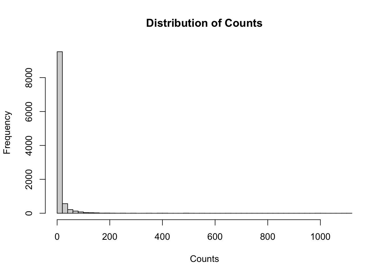
# Histogram for continuous variableshist(data$counts, breaks =40,main ="Distribution of Counts", xlab ="Counts")
The data look pretty zero inflated… as we normally see with ecological counts. Which species were observed most frequently?
# Bar plot for categorical datapar(mar =c(10, 5, 5, 5))barplot(table(data$sppname)|>sort(decreasing =TRUE)|>head(40), main ="Frequency of Categories", xlab =NULL, ylab ="Frequency", las =2)
Best Practices for EDA
Start Broad, Then Narrow: Begin with overall summaries, then dive into specific variables or relationships of interest.
Combine Numerical and Visual Methods: Use both statistical summaries and visualizations for a comprehensive understanding.
Check Data Quality: Always look for missing values, outliers, and unexpected patterns.
Explore Relationships: Look at how different variables relate to each other.
Consider the Context: Interpret your findings in the context of your domain knowledge and research questions.
Document Your Process: Keep notes on your observations and decisions made during EDA.
By following these steps and practices, you’ll gain a thorough understanding of your data, which is crucial for informed decision-making in subsequent analyses.