Descriptive Statistics
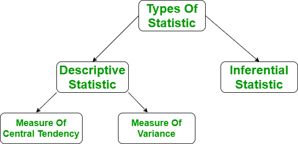
Descriptive statistics form the foundation of data analysis, providing a comprehensive overview of the main characteristics of a dataset. These tools allow us to summarize complex information, identify patterns, and communicate findings effectively.
Measures of Central Tendency
The Mean
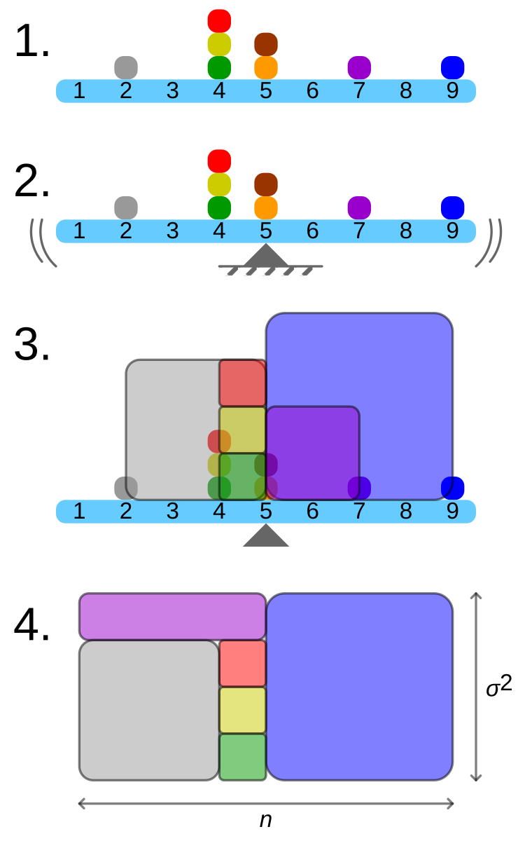
At its core, the mean is a simple concept - add up all your values and divide by how many there are.
\(\bar{y} = \frac{\sum_{i=1}^{n} y_i}{n}\)
Where \(y_i\) is the \(i\)th observation, and \(n\) is the number of observations.
In Excel, you can quickly calculate the mean using =AVERAGE(range), and in R you can use mean(data_vector).
The mean:
provides a single, central value that encapsulates an entire dataset.
is widely understood, making it an excellent tool for communicating findings to diverse audiences.
is heavily used in stats. Many advanced statistical tests, such as t-tests, ANOVA, and regression analysis, rely on the mean as a fundamental descriptive stat. Comparing means between different groups can reveal significant patterns or differences in your data.
However, the mean isn’t without its weaknesses. It can be heavily influenced by outliers, potentially giving a skewed representation of your data. This is where other measures of central tendency come into play.
Median and Mode
The median, the middle value in a sorted dataset, offers a different view of your data’s center. It’s particularly useful when dealing with skewed distributions or datasets with extreme outliers.
Case Study: Household Income

A prime example of the median’s usefulness is in reporting household income. In many countries, income distributions are right-skewed, meaning there’s a long tail of high-income earners that can significantly inflate the mean.
For instance, a study by the U.S. Census Bureau in 2019 reported the following for household income:
- Mean household income: $98,088
- Median household income: $68,703
(U.S. Census Bureau, 2020)
The substantial difference between these two measures highlights the skewed nature of income distribution. The mean is pulled upward by a small number of very high-income households, while the median provides a more representative measure of a “typical” household’s income.
This case underscores why economists and policymakers often prefer the median when discussing household income. It’s less sensitive to extreme values and thus gives a clearer picture of the economic situation for the majority of households.
The mode, the most frequently occurring value, is mostly used in categorical data analysis. In fields like marketing or social sciences, understanding the most common response or characteristic can be crucial for decision-making.
Measures of Dispersion
“If a statistician had her hair on fire and her feet in a block of ice, she would say that ‘on the average’ she felt good.”
While measures of central tendency give us a sense of the typical value in our dataset, measures of dispersion tell us how spread out our data is (or in the case of the statistician, the extremes of temperature felt from head to toe. This spread can often be just as important as the center.
Variance
Variance quantifies how far a set of numbers are spread out from their average value. It’s calculated as:
\(s^2 = \frac{\sum_{i=1}^{n} (y_i - \bar{y})^2}{n-1}\)
The importance of variance lies in its ability to capture the overall variability in a dataset. A larger variance indicates more spread-out data, while a smaller variance suggests the data points are clustered closer to the mean. This concept is crucial in fields ranging from finance (where variance is used to measure risk) to quality control in manufacturing (where consistent, low-variance processes are desirable).
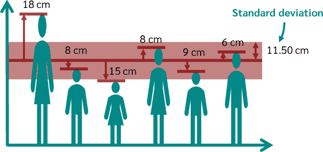
Standard Deviation
excerpt from Descriptive Statistics by Jay Hill
As useful as variance is as a measure, it poses a slight problem. When you are using variance you are dealing with squares of numbers. That makes it a little hard to relate the variance to the original data. So, how can you “undo” the squaring that took place earlier?
The way most statisticians choose to do this is by taking the square root of the variance. When this brilliant maneuver was made the great statistics gods named the new measurement standard deviation and it was good and the name stuck.
\(s = \sqrt{\frac{\sum_{i=1}^{n} (y_i - \bar{y})^2}{n-1}}\)
In Excel, you can use =STDEV(range) for sample standard deviation or =STDEV.P(range) for population standard deviation. R users can use sd(data_vector).
The standard deviation is particularly valuable because:
It’s expressed in the same units as your original data, making it more intuitive to interpret.
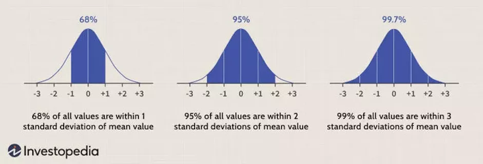
It provides a consistent way to describe the spread of your data. For normally distributed data, about 68% of values fall within one standard deviation of the mean, 95% within two, and 99.7% within three.
In many fields, from psychology to environmental science, results are often reported in terms of standard deviations from the mean.
Standard Error of the Mean (SEM)
excerpt from Handbook of Biologicial Statistics, by John McDonald
When you take a sample of observations from a population and calculate the sample mean, you are estimating of the parametric mean, or mean of all of the individuals in the population. Your sample mean won’t be exactly equal to the parametric mean that you’re trying to estimate, and you’d like to have an idea of how close your sample mean is likely to be. If your sample size is small, your estimate of the mean won’t be as good as an estimate based on a larger sample size. Here are 10 random samples from a simulated data set with a true (parametric) mean of 5. The X’s represent the individual observations, the red circles are the sample means, and the blue line is the parametric mean.
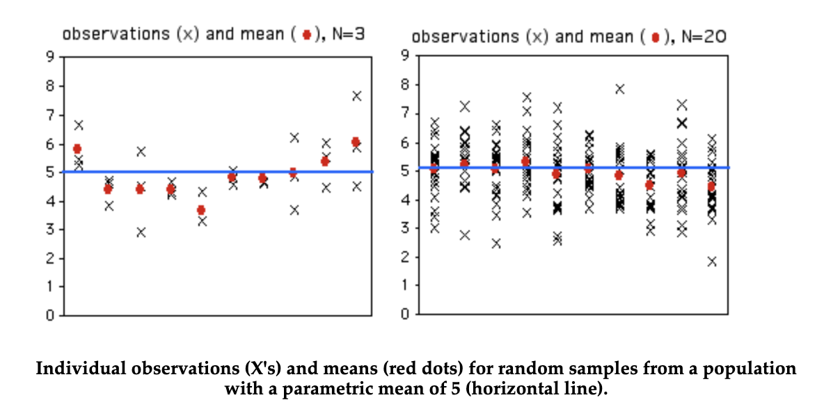
As you can see, with a sample size of only 3, some of the sample means aren’t very close to the parametric mean. The first sample happened to be three observations that were all greater than 5, so the sample mean is too high. The second sample has three observations that were less than 5, so the sample mean is too low. With 20 observations per sample, the sample means are generally closer to the parametric mean.
Once you’ve calculated the mean of a sample, you should let people know how close your sample mean is likely to be to the parametric mean. One way to do this is with the standard error of the mean. If you take many random samples from a population, the standard error of the mean is the standard deviation of the different sample means. About two-thirds (68.3%) of the sample means would be within one standard error of the parametric mean, 95.4% would be within two standard errors, and almost all (99.7%) would be within three standard errors.
The equation for the standard error of the mean is:
\(\text{SEM} = \frac{s}{\sqrt{n}}\)
In Excel, you can calculate this with =STDEV.S(range)/SQRT(COUNT(range)), while in R, you might use sem <- sd(data) / sqrt(length(data)).
The SEM is invaluable because:
It helps us understand how well our sample mean estimates the true population mean.
It’s used in calculating confidence intervals, allowing us to make statements about the range in which we expect the true population parameter to fall.
As sample size increases, the SEM decreases, reflecting our increased confidence in larger samples.
Test Your Understanding
Quiz: Descriptive Statistics
1. Which measure of central tendency is most affected by extreme outliers?
a) Meanb) Median
c) Mode
2. What does the standard deviation represent?
a) The average value in a datasetb) The middle value in a dataset
c) The average distance from the mean
3. Which of the following is true about the variance?
a) It's always positiveb) It's in the same units as the original data
c) It's the square root of the standard deviation
4. What does SEM stand for?
a) Standard Error Measurementb) Standard Error of the Mean
c) Sample Estimation Method
5. As sample size increases, what happens to the Standard Error of the Mean?
a) It increasesb) It decreases
c) It remains the same