Random Effects ANOVA

Understanding Random Effects

When designing experiments, we often encounter factors that aren’t fixed or predetermined. Instead, these factors represent a random sample from a broader population of possible levels. This is where random effects come into play. They allow us to model and account for variability that isn’t due to the fixed factors we’re studying directly.

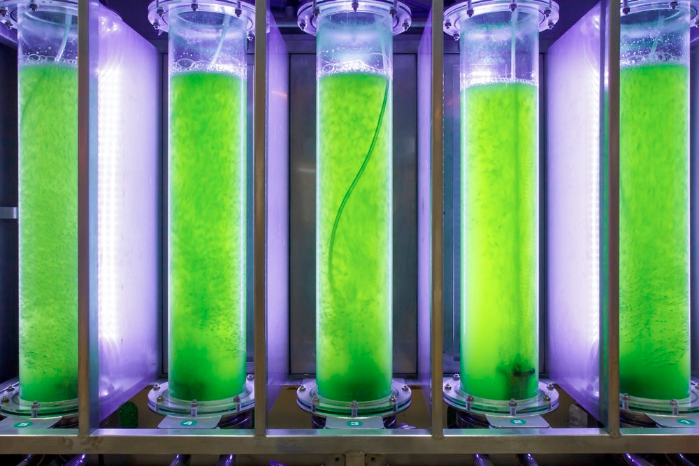
Consider a study on algae growth under different light conditions. While the light levels are fixed (we choose specific intensities), the tanks we use might be randomly selected from a larger set of available tanks. In this case, “tank” becomes our random effect.

The Null Hypothesis in Random Effects ANOVA

In a random effects model, our null hypothesis takes a slightly different form. Instead of testing for differences between specific group means, we’re interested in whether the random effect explains any variability in our dependent variable. Essentially, we’re asking: “Does the random factor (e.g., tank) contribute significantly to the variation we observe in our outcome?”

For random effects, the null hypothesis states that the random effect does not explain any of the variability in the dependent variable. In other words, the random factor doesn’t significantly affect the outcome we’re measuring.

The null hypothesis for the main effect is the same, that is, the null hypothesis states that there is no difference between the means of the groups.

Implementing Random Effects ANOVA

Let’s walk through an example to see how we can implement a random effects ANOVA in R. We’ll use a simulated dataset examining algae growth rates under different light conditions, with multiple tanks for each condition.

Data Simulation

First, we’ll create our dataset:

# set.seed(123)
# df_rand <- data.frame(
#   growth_rate = c(rnorm(60, mean=15, sd=2), rnorm(60, mean=20, sd=2)),
#   light_condition = rep(c("Low", "High"), each=60),
#   tank = rep(1:12, times=10)
# )

# Set seed for reproducibility
set.seed(123)

# Number of tanks and observations per tank
num_tanks <- 10
obs_per_tank <- 15

# Generate tank effects (random effect)
tank_effects <- rnorm(num_tanks, mean = 0, sd = 2)

# Generate light condition effects (fixed effect)
light_effects <- c("Low" = 0, "Medium" = 3, "High" = 6)

# Create the dataset
df_rand <- data.frame(
  tank = rep(1:num_tanks, each = obs_per_tank),
  light_condition = rep(rep(c("Low", "Medium", "High"), each = obs_per_tank/3), num_tanks)
)

# Generate growth rates
df_rand$growth_rate <- with(df_rand, 
  15 + # base growth rate
  tank_effects[tank] + # random effect of tank
  light_effects[light_condition] + # fixed effect of light
  rnorm(nrow(df_rand), mean = 0, sd = 1) # random noise
)

# Convert factors
df_rand$tank <- as.factor(df_rand$tank)
df_rand$light_condition <- factor(df_rand$light_condition, levels = c("Low", "Medium", "High"))

# Display the first few rows
head(df_rand)

  tank light_condition growth_rate
1    1             Low    15.10313
2    1             Low    14.23886
3    1             Low    14.27982
4    1             Low    13.98973
5    1             Low    13.32321
6    1          Medium    18.66596

# Summary statistics
summary(df_rand)

      tank    light_condition  growth_rate   
 1      :15   Low   :50       Min.   :11.45  
 2      :15   Medium:50       1st Qu.:15.43  
 3      :15   High  :50       Median :18.11  
 4      :15                   Mean   :18.13  
 5      :15                   3rd Qu.:20.44  
 6      :15                   Max.   :26.62  
 (Other):60

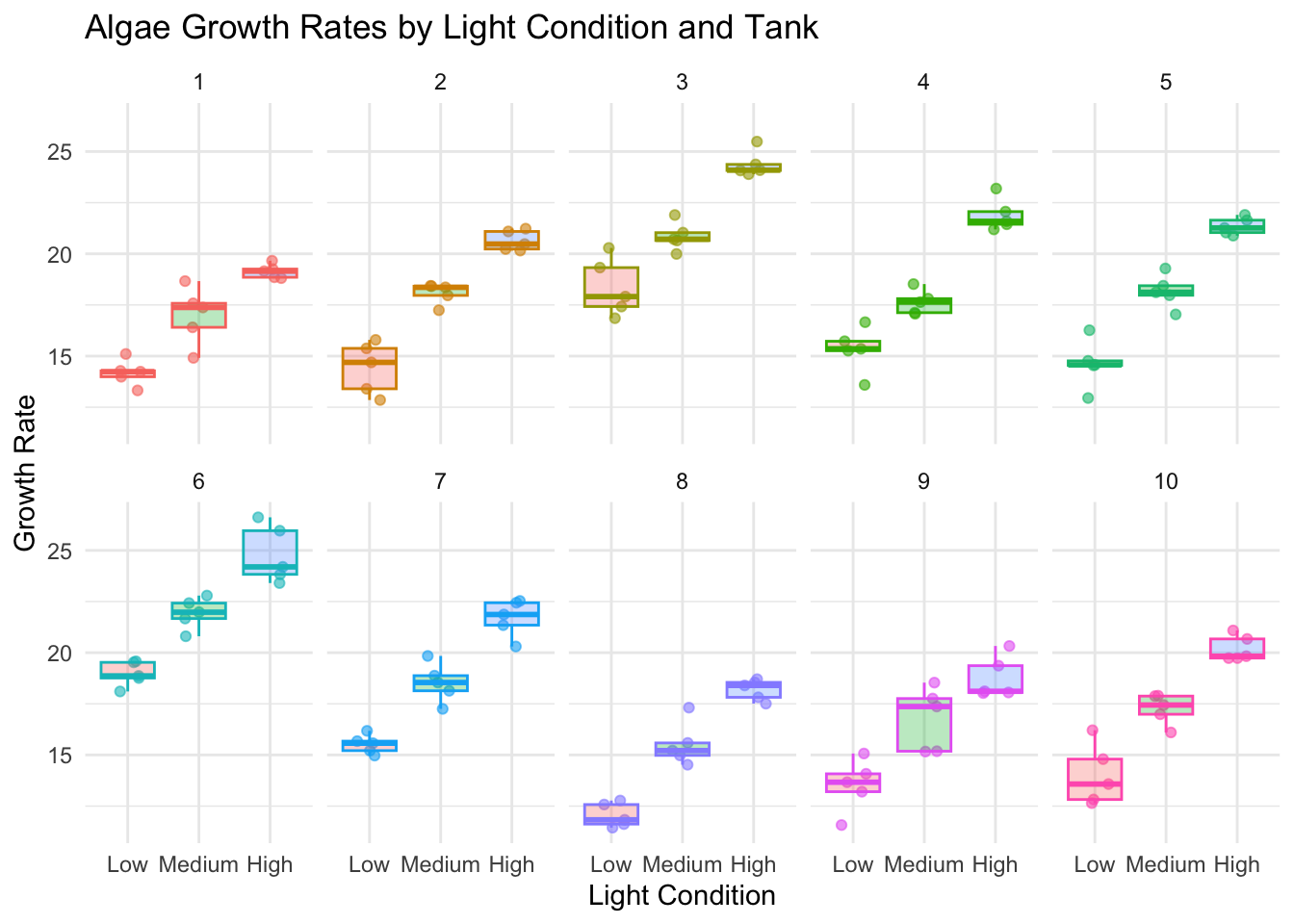
# Plot to visualize the data
library(ggplot2)

ggplot(df_rand, aes(x = light_condition, y = growth_rate, color = tank)) +
  geom_jitter(width = 0.2, alpha = 0.6) +
  geom_boxplot(aes(fill = light_condition), alpha = 0.3, outlier.shape = NA) +
  facet_wrap(~tank, ncol = 5) +
  theme_minimal() +
  labs(title = "Algae Growth Rates by Light Condition and Tank",
       x = "Light Condition", y = "Growth Rate") +
  theme(legend.position = "none")

This dataset represents growth rates for algae in 12 different tanks, split between low and high light conditions.

Model Formulation

Now, let’s create our random effects model:

model_aov <- aov(growth_rate ~ light_condition + Error(tank), data = df_rand)

The key part of our random effects model is the Error(tank) term. This tells R to treat ‘tank’ as a random effect, accounting for the variability between tanks that isn’t explained by the light conditions.

lets run a model without the random effect to compare the variance accounted for by the random effect

model_aov_norand <- aov(growth_rate ~ light_condition, data = df_rand)

Interpreting the Results

Let’s look at the output of our random effects model:

summary(model_aov)


Error: tank
          Df Sum Sq Mean Sq F value Pr(>F)
Residuals  9    573   63.67               

Error: Within
                 Df Sum Sq Mean Sq F value Pr(>F)    
light_condition   2  903.7   451.8     513 <2e-16 ***
Residuals       138  121.5     0.9                   
---
Signif. codes:  0 '***' 0.001 '**' 0.01 '*' 0.05 '.' 0.1 ' ' 1

This output gives us two main sections:

Error: tank: This shows the variability associated with our random effect (tank).
Error: Within: This shows the effects of our fixed factor (light_condition) and the residual variability.

The lack of an F-value or p-value for the random effect is normal in this type of output. To assess the importance of the random effect, we can compare models with and without the random effect.

summary(model_aov_norand)

                 Df Sum Sq Mean Sq F value Pr(>F)    
light_condition   2  903.7   451.8   95.63 <2e-16 ***
Residuals       147  694.6     4.7                   
---
Signif. codes:  0 '***' 0.001 '**' 0.01 '*' 0.05 '.' 0.1 ' ' 1

Comparing our random effects model with the simpler model reveals crucial insights about our algae growth experiment. Both show that light significantly affects growth, but the random effects model tells a more complete story.

The random effects model partitions variance between and within tanks, uncovering an important source of variability we’d otherwise miss. The dramatically lower residual variance (0.9 vs 4.7) in this model shows that much of what seemed like unexplained variation is actually due to tank differences.

Key differences between the models:

• F-value for light condition: 513 (random effects) vs 95.63 (simple model)

This stark contrast in F-values is telling. By accounting for tank variability, we’ve greatly increased our statistical power to detect light’s effect on algae growth.

Including tank as a random factor changes how we interpret our experiment. We’re no longer limited to these specific tanks; we can think more broadly about tanks in general. This approach respects the nested structure of our data - observations within a tank aren’t truly independent.

The random effects model provides a more accurate picture of our experiment by:

Acknowledging complex sources of variation
Increasing our ability to detect true effects
Allowing for broader generalization of results

In short, while both models highlight light’s importance in algae growth, the random effects model offers a more nuanced understanding. It reminds us that in biological systems, unmeasured factors like tank variability can significantly impact our results.

Visualization

To better understand our data, let’s create a visualization:

library(ggplot2)

# Create an improved plot
p_rand_improved <- ggplot(df_rand, aes(x = light_condition, y = growth_rate)) +
  # Add individual points, colored by tank
  geom_jitter(aes(color = tank), width = 0.2, alpha = 1) +
  # Add boxplots
  geom_boxplot(fill = "black",alpha = 0.7, outlier.shape = NA) +
  # Customize colors
  scale_color_viridis_d(option = "plasma") +
  # scale_fill_viridis_d(option = "viridis", alpha = 0.3) +
  # Customize labels and theme
  labs(x = "Light Condition", 
       y = "Algae Growth Rate (g/day)", 
       color = "Tank",
       caption = stringr::str_wrap("Algae growth rates under different light conditions, colored by tank. The boxplots show the distribution of growth rates within each light condition, including median and interquartile ranges, with individual data points overlaid for each tank.")) +
  theme_minimal() +
  theme(legend.position = "right",
        plot.title = element_text(hjust = 0.5, face = "bold"),
        axis.title = element_text(face = "bold"),
        legend.title = element_text(face = "bold"))

# Display the plot
print(p_rand_improved)

This boxplot helps us visualize the differences in growth rates between light conditions, while also showing the spread of the data, which partly reflects the variability between tanks.

Overall Impact on Main Effects

Random effects structures can both increase and decrease the significance of main effects terms.

The inclusion of random effects accounts for variability in the data that isn’t captured by the fixed effects.

Depending on the nature of this variability, the significance of main effects can be influenced in both directions.

Increase the Significance of Main Effects:

When a random effect accounts for a substantial amount of variability that’s unexplained by the main effects, including this random effect can lead to a clearer pattern in the fixed effect, increasing its significance.

Example: Imagine studying the growth rate of algae across different oceans (Pacific, Atlantic, Indian). Within each ocean, multiple samples are taken at different depths (randomly selected). If the variability between depths is significant and not accounted for, it can obscure the true difference in growth rates between oceans. By including depth as a random effect, the variability due to depth is accounted for, potentially revealing a clearer difference in growth rates between oceans.
Decrease the Significance of Main Effects:

If the variability attributed to the random effect overlaps with the variability attributed to the main effect, the significance of the main effect might decrease. This happens because the random effect “absorbs” some of the variability initially thought to be due to the main effect.

Example: Consider an experiment measuring fish metabolism at different temperatures (warm, cold) across various tanks. Suppose the temperatures aren’t perfectly controlled, and some tanks naturally run warmer than others. If “tank” is not included as a random effect, we might see a significant difference between warm and cold treatments. However, if “tank” is introduced as a random effect and it captures a significant amount of the temperature variability (because some tanks are naturally warmer), the significance of the temperature effect might decrease.

In both scenarios, the random effects structure helps provide a more accurate representation of the underlying patterns in the data by accounting for unobserved variability. It’s essential to understand the sources of variability in the experiment and consider both fixed and random effects appropriately.

Mixed-Effects Models

A more direct and modern approach to assess the significance of random effects is to fit a linear mixed-effects model (using packages like lme4 or nlme). The significance of random effects can be more directly assessed by comparing a model with the random effect to one without it using likelihood ratio tests.

To learn more about the lmer4 and mixed effects models, check out: