Activity: Millepora in the Gulf of Panama
background

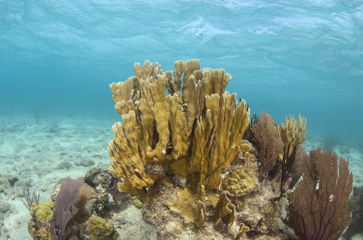
In the vibrant and diverse ecosystems of coral reefs in the gulf of Panama, a research team embarked on a journey to unravel the mysteries of fire coral, Millepora, densities across different habitats and sites. These islands, with their pristine waters and a variety of marine habitats, offer a perfect natural laboratory to explore how environmental variables might influence coral populations.
In this hypothetical study:
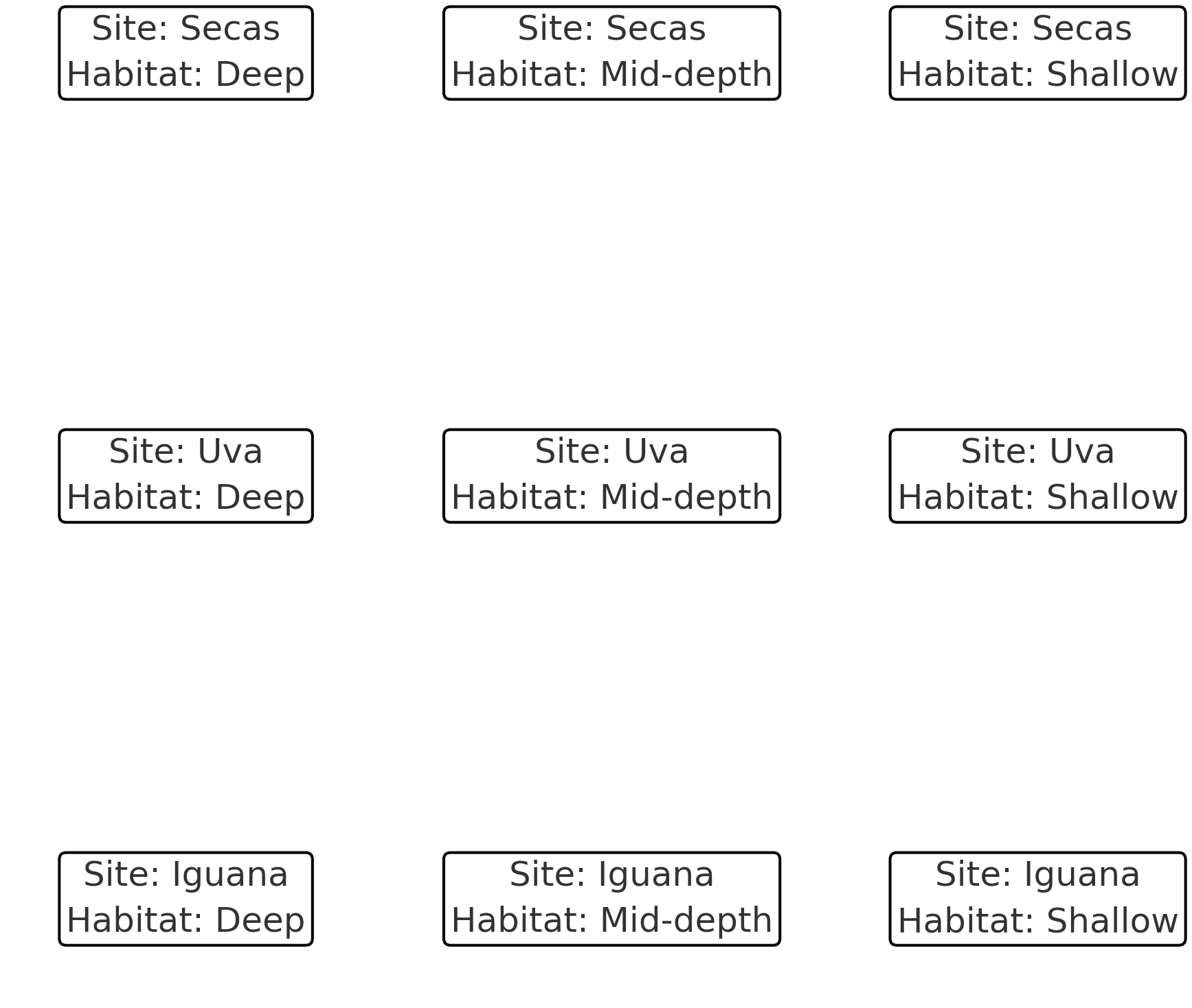
Sites represent distinct geographical locations around the Gulf of Panama, each with its unique marine environmental characteristics and potential human and natural impacts. Differences between sites might be driven by factors like proximity to human activities, ocean currents, or historical disturbances.
Habitats are categorized into “Shallow” , “Deep” , and “Mid-depth,” providing a categorical distinction based on water depth. This might reflect differences in light availability, pressure, and species interactions, which are known to influence coral physiology and distribution.
Millepora Density (colonies per unit area) is the response variable, providing a quantifiable metric to explore the population density of Millepora corals across different conditions. Densities might be influenced by factors like resource availability, predation, and competition, which can vary between habitats and sites.
In this explorative study, the team systematically quantified Millepora densities across various transects in different habitats and sites, aiming to decipher the potential effects of geographical and environmental variables on coral distribution. The dataset thereby provides a rich context for understanding how these two factors (Site and Habitat) might interact to shape Millepora densities across the vibrant reefs of the Secas islands.
This combination of sites and habitat can be viewed as a factorial “design” (even though these are natural surveys).
Your task is to analyze the data from these surveys and determine whether and how Millepora densities differed across sites and habitats.
steps
i. Download the data
Follow the link to Download this data - This will take you to github where you will see option to “Download raw file” on the right side of the window.
ii. Set up your script - you know what to do
1. Import the Data into RStudio. Melt and Rearrange if Necessary.
- Useful commands:
read.csv(),pivot_longer()
2. Describe the Dataset
3. Make a plot of your data
can be any of the types of plots we discussed last week, but consider how you have multiple factors now, so youll also need to look at the examples from this week.
Useful commands:
ggplot(),geom_bar(),geom_errorbar(),geom_boxplot()
4. State the Null Hypotheses for the Two-Way ANOVA of this experiment
- use the exact names of your factors and dependent variable to formulate these hypotheses.
5. Inspect Interaction Between Factors
Use an interaction plot to visualize potential interactions between factors.
Useful commands:
interaction.plot()Does it look to you like there is an interaction in this dataset? why or why not?
6. Perform the Two-Way ANOVA
- Run the ANOVA model including both main effects and the interaction term. (
aov())
7. Test ANOVA Assumptions
- Test for Homogeneity of Variances
- Useful commands:
bartlett.test(),levene.test()
- Check for Normality of Residuals
- Useful commands:
shapiro.test(),qqnorm(),qqline()
8. determine whether transformations are necessary and perform Necessary Data Transformations if so
- briefly (in 2-3 sentences), interpret the outputs of step 7 , and interpret whether or not you should transform the data.
- if assumptions are not met, try different transformations of your data (
log(),sqrt() ) - If you transformed the data, rerun the ANOVA model again and ensure assumptions are met.
9. Report the Results of the Two-Way ANOVA
Generate an ANOVA table. copy the text output from your console into the script so you have the anova table to see and refer to.
Report whether main effects and interactions were significant, and specify the significance level.
Useful commands:
summary(),anova()
10. Perform Post-Hoc Tests if Appropriate and Report the Results
- Useful commands:
TukeyHSD(),HSD.test()fromlibrary(agricolae) - Report which if any pairs were significantly different, and report the significance level. Refer to the previous section in the lab manual on reporting anova results for requirements for post-hoc tests.
11. Create a Graph of Your Data
you may build on the same plot you made in number 3, or try another plot, or build onto it, as long as this plot has all required elements. your plot must also have some kind of error bars and you must define what your error bars mean in your title or caption.
Useful commands:
ggplot(),geom_bar(),geom_errorbar(),facet_wrap(),theme_minimal(), etc.
12. Provide a Short Paragraph (3-4 Sentences) Explaining and interpreting the Results.
- Explain your results statistically, and also interpret them in terms of their ecological importance. Be specific about how Millepora densities varied across the islands and habitats, especially the significant results from post hoc tests, if any were found, and interpret any interactions with respect to these patterns.