More theory and assumptions

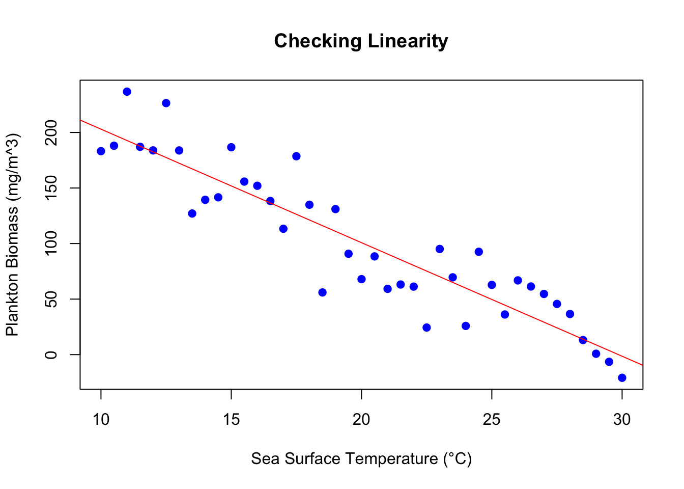
Linear Relationship: Linear regression is built upon the principle that there’s a linear relationship between the independent and dependent variables. This essentially means that the change in the dependent variable can be described by a straight line as the independent variable changes. In a scatter plot, if the data points seem to align along a straight path, this assumption likely holds.

plot(plankton_temp_data$SST, plankton_temp_data$plankton_biomass, 
     xlab="Sea Surface Temperature (°C)", ylab="Plankton Biomass (mg/m^3)",
     main="Checking Linearity", pch=19, col="blue")
abline(lm(plankton_biomass ~ SST, data=plankton_temp_data), col="red")

Types of Linear Regression: While the foundational principle of linear regression is establishing a linear relationship, the complexity of real-world data often means that we’re not just looking at the effect of one variable on another. Sometimes, multiple factors come into play, and it’s essential to understand how they jointly influence an outcome. This brings us to the distinction between Simple and Multiple Linear Regression:

• Simple Linear Regression: This form focuses on describing a relationship between one independent variable and one dependent variable. It’s especially useful when we want to understand and predict outcomes based on a single factor.

\[ Y=β_0+β_1X+ϵ \]

• Multiple Linear Regression: When there are multiple factors or independent variables that might influence the outcome, we turn to multiple linear regression. It helps us understand the collective effect of multiple variables on a dependent variable and can capture more complex relationships in the data. The equation extends to:

\[ Y=β_0+β_1X_1+β_2X_2+...+ϵ \]

---

Null and Alternative Hypotheses

Intercept:

The intercept, represented as \(β_0\), is the expected value of the response variable when all predictor variables are set to zero.

Null Hypothesis for Intercept (\(H_0\)): The expected value of the response variable is zero when all predictor variables are zero.

\[ H_0 : β_0 = 0 \]

Alternative Hypothesis for Intercept (\(H_1\)): The expected value of the response variable is not zero when all predictor variables are zero.

\[ H_1 : β_0 ≠ 0 \]

• If the null hypothesis is rejected (based on a low p-value): There is evidence to suggest that the expected value of the response variable is not zero when all predictors are zero.

• If the null hypothesis is not rejected (based on a high p-value): There isn’t enough evidence to suggest a non-zero expected value of the response variable when all predictors are zero.

Slope:

The slope, represented for a specific predictor as \(β_1\), describes the expected change in the response variable for a one-unit change in the predictor, holding all other predictors constant.

Null Hypothesis for Slope (\(H_0\)): There is no relationship between the predictor and the response variable (i.e., the slope is zero).

\[ H_0 : β_1 = 0 \]

Alternative Hypothesis for Slope (\(H_1\)): There is a relationship between the predictor and the response variable (i.e., the slope is not zero).

\[ H_1 : β_1 ≠ 0 \]

• If the null hypothesis is rejected (based on a low p-value): There is evidence to suggest a significant relationship between the predictor and the response variable.

• If the null hypothesis is not rejected (based on a high p-value): There isn’t enough evidence to suggest a significant relationship between the predictor and the response variable.

---

Assumptions of Linear Regression:

1. Linearity: The foundation of linear regression. We’ve already visualized this with our scatter plot above. The name “linear regression” itself signifies that the relationship is expected to be linear. If the data doesn’t appear linear, transformations or non-linear models might be needed.
2. Independence: Each observation in the dataset is independent of the others. This assumption often requires domain knowledge to validate. For instance, in time-series data, this assumption can be violated because today’s value might depend on yesterday’s. If this assumption is violated, specialized techniques like autoregressive models or random effects might be needed.
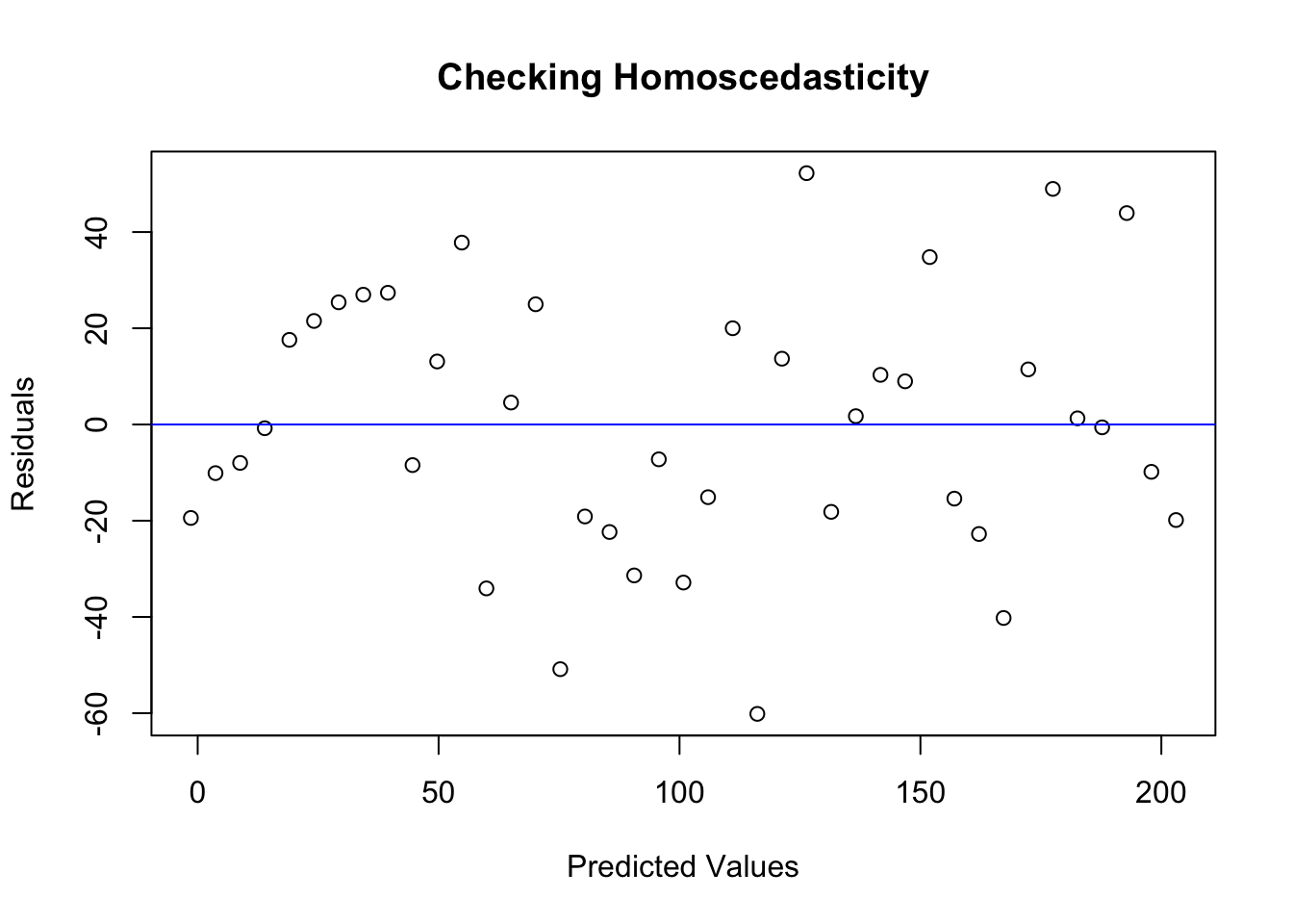
3. Homoscedasticity (Constant Variance): The variance of the residuals remains constant across different levels of the independent variable(s). This can be checked visually using a residuals vs. fitted values plot.

residuals_data <- residuals(model)
predicted_values <- fitted(model)

plot(predicted_values, residuals_data, 
     xlab="Predicted Values", ylab="Residuals",
     main="Checking Homoscedasticity")
abline(h=0, col="blue")

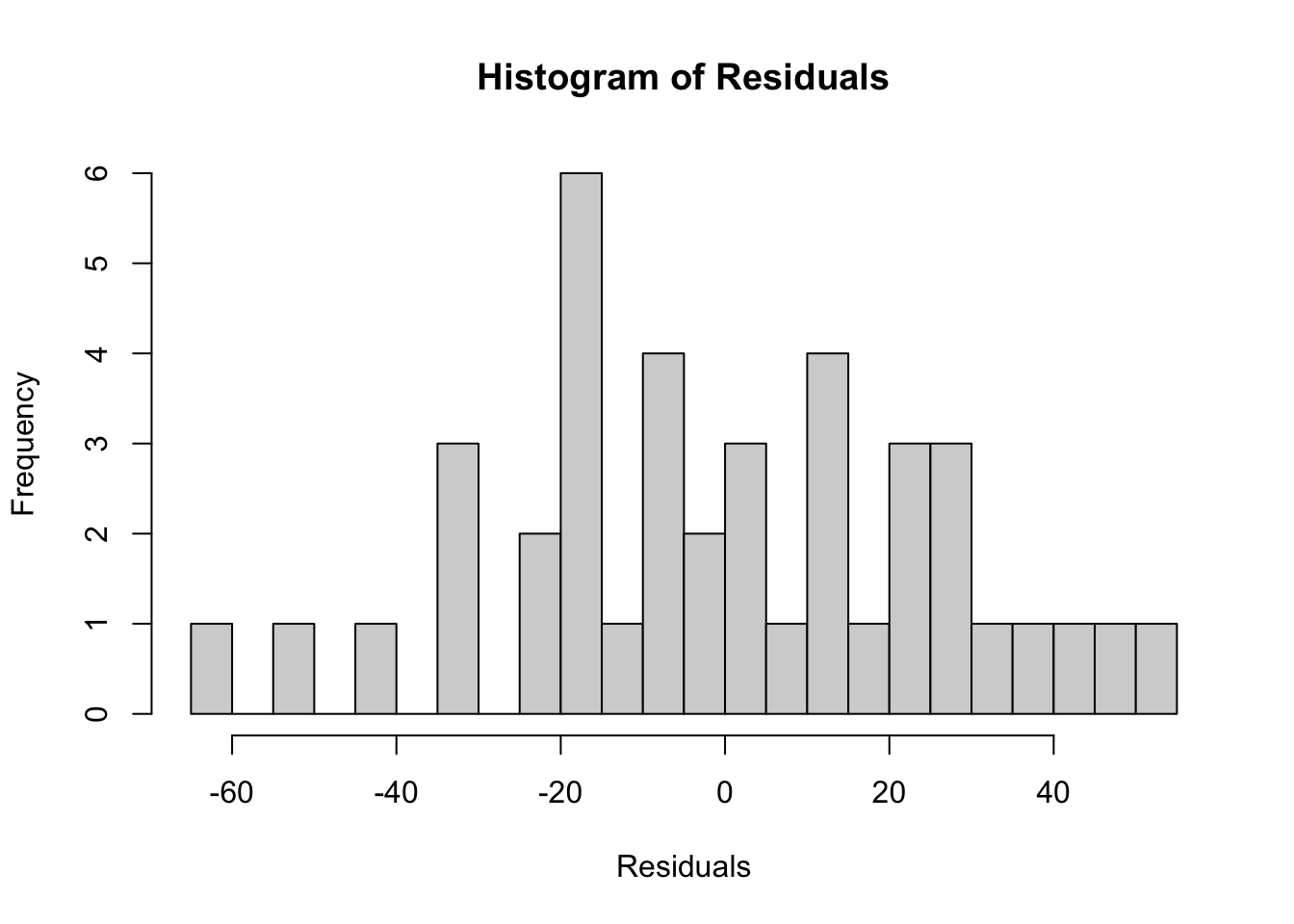
4. Normality of Residuals: For valid hypothesis testing (like testing if coefficients are significant), the residuals should be approximately normally distributed. This can be visually inspected using a histogram or a Q-Q plot.

• Histogram: Outliers or skewness in the histogram can indicate potential violations.

hist(residuals_data, breaks=20, main="Histogram of Residuals", xlab="Residuals")

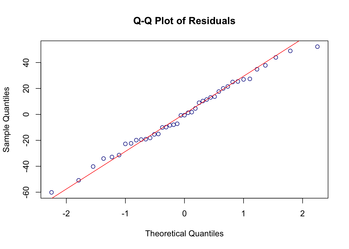
• QQ plot: A Q-Q plot provides a graphical view of how the residuals compare to a normal distribution. If the residuals are normally distributed, the points on the Q-Q plot should lie roughly on a 45-degree straight line.

qqnorm(residuals_data, main="Q-Q Plot of Residuals", col="darkblue")
qqline(residuals_data, col="red")

---

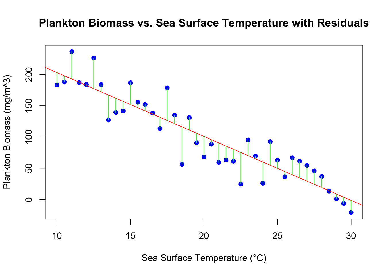
Visualization of Residuals: Understanding residuals is key in regression analysis. Residuals represent the difference between observed and predicted values. These differences should be random and not show patterns. By visualizing residuals using vertical lines, we can get an intuitive feel for the model’s accuracy at different data points.

# Fit the linear regression model
model <- lm(plankton_biomass ~ SST, data = plankton_temp_data)

# Plot the data points
plot(plankton_temp_data$SST, plankton_temp_data$plankton_biomass, 
     xlab="Sea Surface Temperature (°C)", ylab="Plankton Biomass (mg/m^3)",
     main="Plankton Biomass vs. Sea Surface Temperature with Residuals",
     pch=19, col="blue")

# Add the regression line
abline(model, col="red")

# Draw vertical lines for residuals
predicted_values <- fitted(model)
segments(plankton_temp_data$SST, plankton_temp_data$plankton_biomass, plankton_temp_data$SST, predicted_values, col="green")