Covariance

Covariance is a fundamental statistical concept that measures how two variables change together. It provides insight into the direction of the linear relationship between variables but doesn’t indicate the strength of that relationship. The formula for covariance is:

\[\sigma_{XY} = \frac{\sum_{i=1}^{n}(X_i - \mu_X)(Y_i - \mu_Y)}{n}\]

Where \(X_i\) and \(Y_i\) are individual data points, \(\mu_X\) and \(\mu_Y\) are the means of X and Y respectively, and n is the number of data points.

Covariance can take any value from negative infinity to positive infinity. A positive covariance indicates that as one variable increases, the other tends to increase as well. Conversely, a negative covariance suggests that as one variable increases, the other tends to decrease.

Covariance vs Correlation

While covariance provides valuable information, its scale dependence makes it challenging to interpret in isolation. This is where correlation comes in. Correlation is essentially a standardized form of covariance, calculated by dividing the covariance by the product of the standard deviations of the two variables:

\[r = \frac{\sigma_{XY}}{\sigma_X \sigma_Y}\]

This standardization results in a correlation coefficient that always falls between -1 and 1, making it much easier to interpret and compare across different datasets.

Let’s illustrate these concepts with a simulated dataset:

library(tibble)
library(ggplot2)

set.seed(123)

ocean_data <- data.frame(
  ocean_temp = rnorm(100, mean = 20, sd = 5),
  plankton_count = rnorm(100, mean = 500, sd = 100)
)

# Calculating covariance
cov_value <- cov(ocean_data$ocean_temp, ocean_data$plankton_count)
print(paste("Covariance:", cov_value))

[1] "Covariance: -21.8605359137837"

# Calculating correlation
cor_value <- cor(ocean_data$ocean_temp, ocean_data$plankton_count)
print(paste("Correlation:", cor_value))

[1] "Correlation: -0.049532147170365"

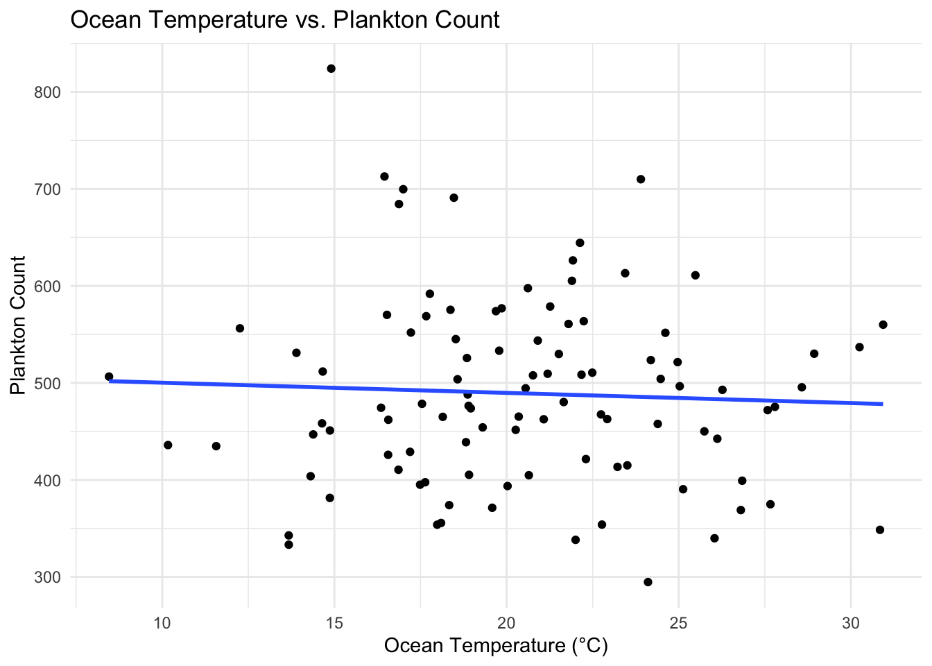
In this example, the covariance value (-21.86054) indicates a negative relationship between ocean temperature and plankton count. However, the magnitude of this value is difficult to interpret without context. The correlation coefficient (-0.04953215) provides a clearer picture, suggesting a very weak negative relationship between these variables.

ggplot(ocean_data, aes(x = ocean_temp, y = plankton_count)) +
  geom_point() +
  geom_smooth(method = "lm", se = FALSE) +
  theme_minimal() +
  labs(title = "Ocean Temperature vs. Plankton Count",
       x = "Ocean Temperature (°C)",
       y = "Plankton Count")

This scatter plot visually represents the relationship captured by our covariance and correlation calculations. The slight downward slope of the trend line corresponds to the negative covariance and correlation we observed.

Considerations and Limitations

In fields studying complex systems, such as ecology or climatology, relationships between variables are often non-linear and influenced by multiple factors. In these cases, more advanced techniques like partial correlation, multiple regression, or non-parametric methods might be necessary to fully understand the relationships in the data.

Summary

Differences between covariance and correlation:

Magnitude and Scale:
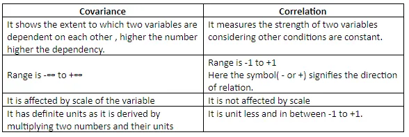
- Covariance can take on any value between negative infinity and positive infinity, making it difficult to interpret on its own. Its value is influenced by the scale of the variables.
- Correlation, on the other hand, is dimensionless and ranges between -1 and 1, providing a standardized measure of association.
Interpretability:
- Covariance only indicates the direction of the linear relationship between variables (positive or negative). It doesn’t convey the strength of that relationship.
- Correlation quantifies both the strength and direction of the linear relationship.
Units:
- Covariance is measured in units that are the product of the units of the two variables.
- Correlation has no units; it’s a pure value.