Chi-square: Understanding Categorical Data Analysis
Foundations of Chi-square Testing
The chi-square test helps us analyze categorical data through goodness-of-fit and independence testing. Before starting any analysis, your data must meet two key requirements:
Independent observations: The classification of one observation shouldn’t influence another
Adequate sample size: No more than 20% of categories should have expected frequencies below 5
review
conditions for chi-square
observations are independent
no more than 20% of the categories have expected frequencies < 5
We measure differences between observed and expected patterns using the chi-square statistic (\(\chi^2\)): \(\chi^2 = \sum \frac{(O - E)^2}{E}\). This calculation squares the differences, ensuring all deviations contribute positively and giving extra weight to larger discrepancies.
Understanding the Chi-square Distribution
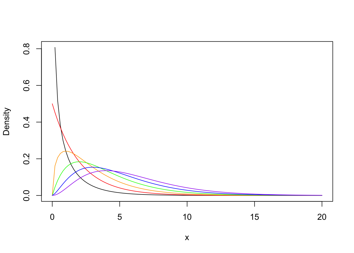
curve(dchisq(x, df =1), 0, 20, ylab ="Density")curve(dchisq(x, df =2), add =T, col ="red")curve(dchisq(x, df =3), add =T, col ="orange")curve(dchisq(x, df =4), add =T, col ="green")curve(dchisq(x, df =5), add =T, col ="blue")curve(dchisq(x, df =6), add =T, col ="purple")
The chi-square distribution reveals how likely your results are to occur by chance. In the plot above, each curve represents a different degrees of freedom (df), shown in different colors from red (df=2) to purple (df=6). As df increases, the peak shifts right and the curve flattens out. The x-axis shows your chi-square statistic - higher values suggest your observed data is less likely under the null hypothesis. To find your p-value, calculate the area under your df’s curve to the right of your statistic.
Two Approaches to Chi-square Testing
Chi-square testing takes two main forms, each answering different research questions. The goodness-of-fit test compares one variable’s frequencies against theoretical expectations. For example, testing whether coin flip results match an expected 50-50 split. The degrees of freedom are calculated as k-1, where k is the number of categories.
The independence test examines relationships between two variables, like testing whether education level relates to voting patterns. Here, degrees of freedom are calculated as (r-1)(c-1), where r and c represent the rows and columns in your data table.
Both approaches share common elements:
Use the chi-square statistic and distribution
Work with categorical data
Compare observed versus expected frequencies
Choose your approach based on your research question: goodness-of-fit for testing against theoretical expectations, independence testing for examining relationships between variables.