Analysis of Covariance (ANCOVA)
Foundations and Purpose
Analysis of covariance (ANCOVA) combines the features of ANOVA and regression into a powerful statistical approach. By incorporating continuous variables (covariates) into the analysis of group differences, ANCOVA provides a more refined understanding of relationships in your data.
When comparing groups, underlying continuous variables called covariates often influence your dependent variable. ANCOVA accounts for these influences by adjusting group means based on the covariates, leading to more precise comparisons. Think of it as “leveling the playing field” before comparing groups.
Covariates
A covariate is a continuous variable that potentially influences your dependent variable but isn’t the main focus of your study. Think of it as background variation you want to control for. For example, if you’re comparing growth rates between treatment groups, initial size might be a covariate - it affects growth but isn’t your primary interest. By including covariates in your analysis, you can often explain more variation in your data and reveal patterns that might otherwise be hidden.
Hypotheses
ANCOVA tests have a few components to their hypotheses:
- Main Effect
- H₀: No differences exist between group means after adjusting for the covariate
- H₁: At least one group mean differs from others after adjusting for the covariate
- Covariate Effect
- H₀: There is no linear relationship between the covariate and the dependent variable
- H₁: There is a linear relationship between the covariate and the dependent variable
For example, when studying shark swimming speeds (as we do in the next section):
Main effect H₀: No difference in swimming speeds between species after accounting for temperature
Covariate H₀: Water temperature has no effect on swimming speed
Slopes H₀: The effect of temperature on swimming speed is the same for both species
Mathematical Framework
The ANCOVA model builds upon the ANOVA framework by adding a regression component. The general linear model is expressed as:
\[ Y_{ij} = \mu + \tau_i + \beta(X_{ij} - \bar{X}) + \epsilon_{ij} \]
In this equation, \(Y_{ij}\) represents the dependent variable for each observation, \(\mu\) is the overall mean, and \(\tau_i\) captures the effect of different groups. The covariate effect is represented by \(\beta(X_{ij} - \bar{X})\), where \(\beta\) is the regression coefficient, \(X_{ij}\) is the covariate value, and \(\bar{X}\) is the covariate mean. Random error is denoted by \(\epsilon_{ij}\).
Understanding Variance Partitioning
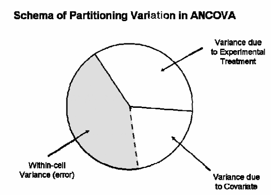
ANCOVA’s power lies in its ability to partition variance more effectively than ANOVA. By accounting for covariate effects, ANCOVA reduces unexplained variance, leading to more sensitive statistical tests. This partitioning has several key benefits:
The statistical power increases when relevant covariates are included, as the Mean Square Error (MSerror) typically decreases. This reduction results in larger F values and smaller p-values, improving your ability to detect true effects when they exist.
ANCOVA enhances precision by controlling for sources of variation that might otherwise mask treatment effects. This control is particularly valuable when random assignment isn’t possible or when you need to account for pre-existing differences between groups.
Assumptions
Independence and Random Sampling
Observations must be independent both within and across groups. This assumption stems from study design and sampling methods rather than statistical tests. Read more here.
Homogeneity of Variances
The variability in your dependent variable should be similar across all groups. You can test this using Bartlett’s test or Levene’s test:
Normality of Residuals
Residuals should follow a normal distribution within each group.
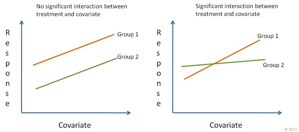
Homogeneity of Regression Slopes (a new assumption!!)
The covariate’s effect should be consistent across all groups. Test this by including an interaction term between your covariate and independent variable. A non-significant interaction suggests this assumption is met.