Question Addressed: What is the degree of association between two variables?
Key Point: One variable might be the cause of the other, but correlation analysis does not make this assumption. It’s possible that both variables are the effects of a common cause.
In correlation analysis, the null hypothesis \(H_0\) posits that there’s no association between the two variables, meaning the correlation coefficient \(r\) is 0. If the p-value from the correlation test is less than a significance level (commonly 0.05), then we reject the null hypothesis. This would suggest that there’s a statistically significant correlation between the two variables.
In our example with coral_data, if the p-value is less than 0.05, we would conclude that there’s a statistically significant correlation between Sea Surface Temperature and Coral Mortality Rate.
Assumptions
For Pearson’s correlation to be valid, certain assumptions about the data need to be met. One in particular is :
Bivariate Normal Distribution:
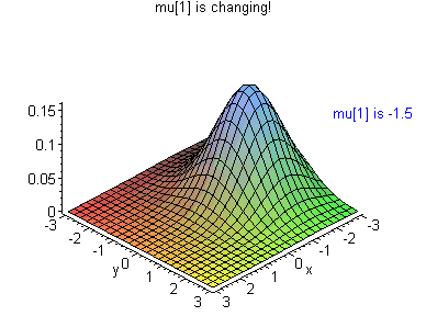
a bivariate normal distribution with a moving mean (source)
The variables under consideration should be “bivariate normal.” This means that each individual variable should be normally distributed, and their relationship should be linear. Non-linear relationships indicate that the bivariate normal distribution assumption doesn’t hold.
Before conducting correlation analysis, it’s essential to test the assumptions.
# Testing for normality in SSTshapiro.test(coral_data$SST)
    Shapiro-Wilk normality test

data:  coral_data$SST
W = 0.99473, p-value = 0.8659
# If p-value < 0.05, SST data is not normally distributed. Consider transformation.# Testing for normality in Coral_Mortality_Rateshapiro.test(coral_data$Coral_Mortality_Rate)
    Shapiro-Wilk normality test

data:  coral_data$Coral_Mortality_Rate
W = 0.99089, p-value = 0.4476
# If p-value < 0.05, Coral_Mortality_Rate data is not normally distributed. Consider transformation.
in both of these cases, assumptions are met!
However, if the assumptions do not hold, transformations can be applied (similar to transformations for anova)
In this example, we applied a log transformation to the Coral_Mortality_Rate variable. This can help normalize the data and meet the assumption of bivariate normality. Note we also applied a +1 to avoid taking the log of zero or negative values.
However, since the shapiro test showed that the data is normally distributed, we will not use the transformed data (this is just an example for you)
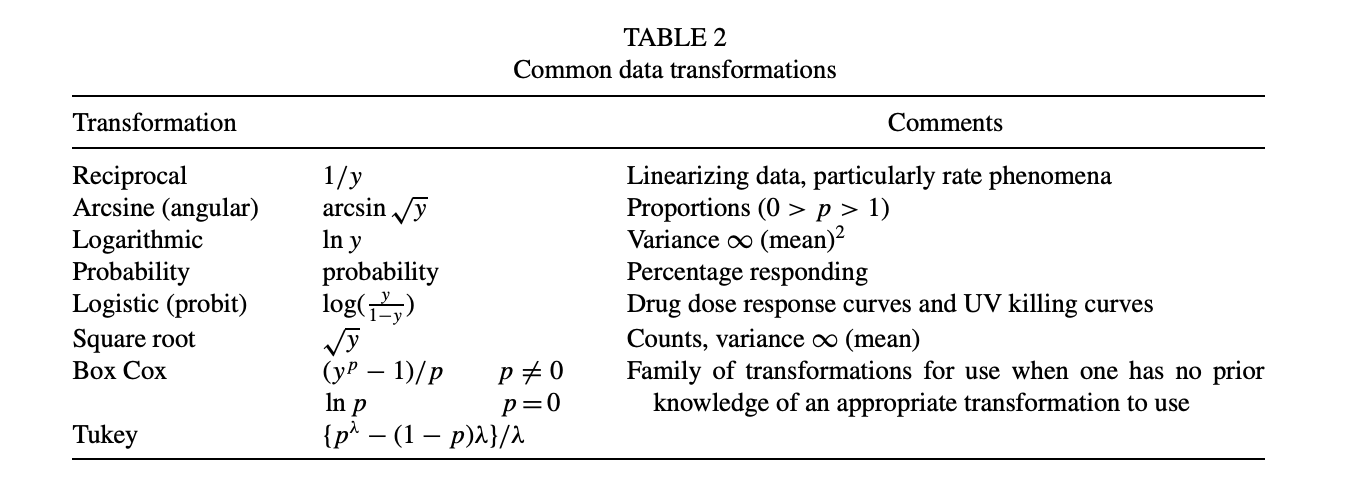
source: table 2 from Asuero, Sayago, and González (2006)
Correlation Analysis
Let’s perform correlation analysis on coral_data and understand the relationship between SST and coral mortality rate.
# Calculating correlation and covariance matricescor_matrix<-cor(coral_data, use="all.obs", method="pearson")cov_matrix<-cov(coral_data, use="all.obs")# Correlation test between SST and Coral_Mortality_Ratecorrelation_test<-cor.test(coral_data$SST, coral_data$Coral_Mortality_Rate, method="pearson")correlation_test
    Pearson's product-moment correlation

data:  coral_data$SST and coral_data$Coral_Mortality_Rate
t = 19.886, df = 148, p-value < 2.2e-16
alternative hypothesis: true correlation is not equal to 0
95 percent confidence interval:
 0.8024859 0.8914340
sample estimates:
    cor
0.85304
Interpretation of Pearson’s Correlation Test Output:
Test Type: The test conducted is Pearson’s product-moment correlation. It measures the linear relationship between two continuous variables.
Data: The correlation analysis was performed on the relationship between Sea Surface Temperature (coral_data$SST) and Coral Mortality Rate (coral_data$Coral_Mortality_Rate).
Test Statistic (t): The value of the test statistic is ( t = 19.886 ). This is a measure of how many standard deviations our correlation coefficient (( r )) is from the null hypothesis value (which is 0, indicating no correlation).
Degrees of Freedom (df): The degrees of freedom is ( df = 148 ). This is calculated as the number of data pairs minus 2.
P-value: The p-value is less than ( 2.2 * 10^{-16} ), which is effectively zero. A p-value this small is highly statistically significant.
Alternative Hypothesis: The alternative hypothesis tested is that the true correlation is not equal to 0. Given the extremely small p-value, we reject the null hypothesis in favor of the alternative, indicating that there is a significant correlation between the two variables.
Confidence Interval: The 95% confidence interval for the correlation coefficient is between ( 0.8024859 ) and ( 0.8914340 ). This means we are 95% confident that the true population correlation lies within this interval.
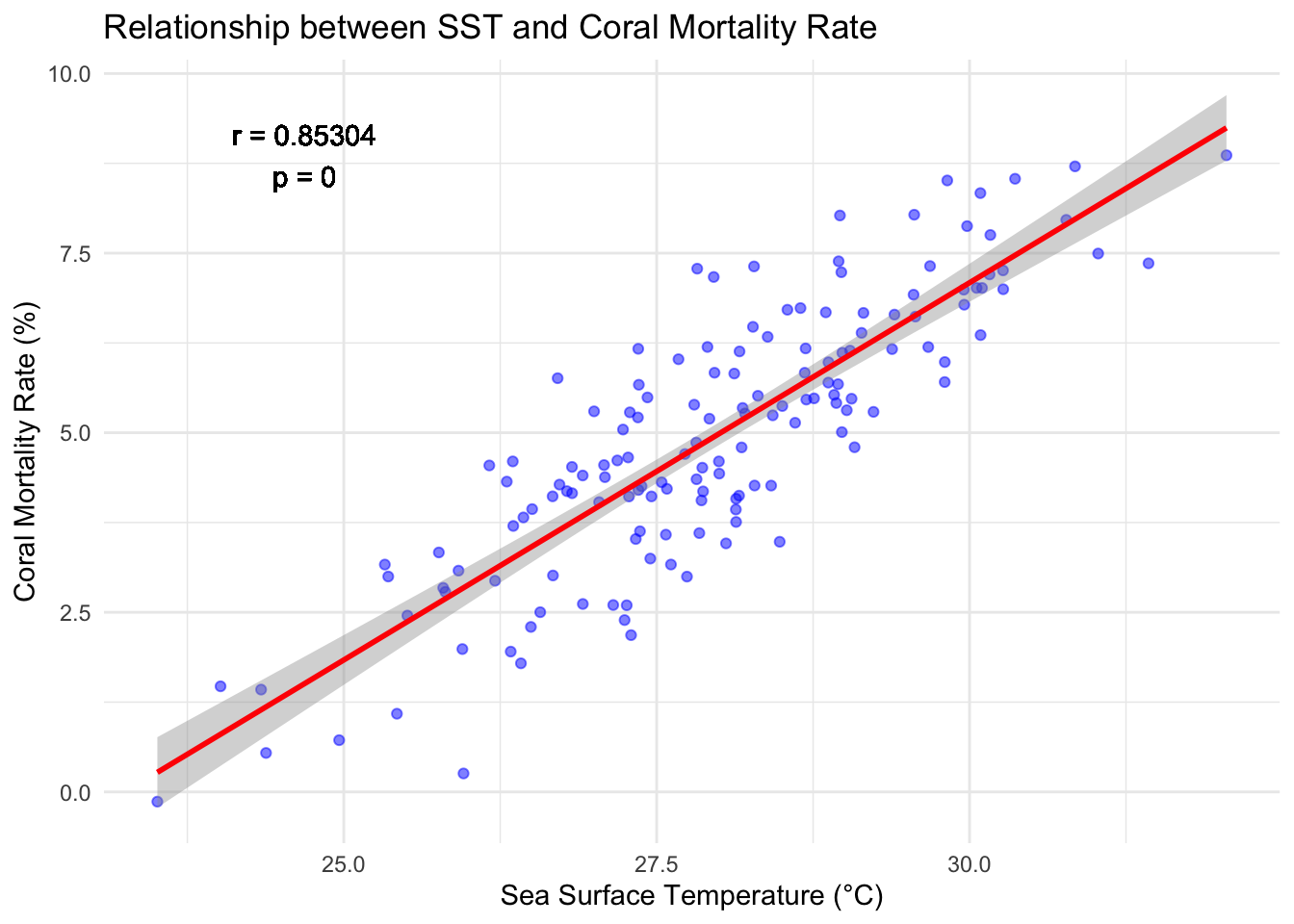
Sample Estimate (( r )): The sample correlation coefficient, ( r ), is ( 0.85304 ). This is a measure of the strength and direction of the linear relationship between the two variables in our sample. Since ( r ) is close to 1, it suggests a strong positive linear relationship between Sea Surface Temperature and Coral Mortality Rate.
In Layman’s Terms: The analysis indicates a strong positive relationship between Sea Surface Temperature and Coral Mortality Rate. As the temperature increases, coral mortality also tends to increase. The strength of this relationship, as indicated by the correlation coefficient of ( 0.85304 ), is quite robust. The statistical test confirms this relationship is significant, with a very low probability (p-value) that the observed relationship happened by chance. The confidence interval further solidifies this result by suggesting that if the study were repeated multiple times, the correlation would likely fall between ( 0.8024859 ) and ( 0.8914340 ) in 95% of the studies.
lets plot!
# Extracting Pearson's r and p-valuer_value<-correlation_test$estimatep_value<-correlation_test$p.value# Plotting the relationship with correlation coefficient and p-value annotationsggplot(coral_data, aes(x =SST, y =Coral_Mortality_Rate))+geom_point(color ="blue", alpha =0.5)+geom_smooth(method ="lm", col ="red")+theme_minimal()+labs(title ="Relationship between SST and Coral Mortality Rate", x ="Sea Surface Temperature (°C)", y ="Coral Mortality Rate (%)")+geom_text(x =min(coral_data$SST)*1.05, y =max(coral_data$Coral_Mortality_Rate), label =paste0("r = ", round(r_value, 6), "\np = ", round(p_value, 4)))
Asuero, A. G., A. Sayago, and A. G. González. 2006. “The Correlation Coefficient: An Overview.”Critical Reviews in Analytical Chemistry 36 (1): 41–59. https://doi.org/10.1080/10408340500526766.