Basic Data Types and Data Structures

Companion Script

Unfold this code to find a companion script

show R code

# ========================================
# Basic Data Types and Data Structures Comprehensive Companion Script
# ========================================

# The difference between data types and data structures:
# Data types refer to the type of data (e.g., numeric, character)
# Data structures refer to how the data is organized (e.g., vectors, matrices)

# ----------------------------------------
# Data Types
# ----------------------------------------

# 1. Numeric: For real numbers (decimal and whole)
x <- 10.5
class(x)  # "numeric"

# 2. Integer: Specifically for whole numbers
y <- 10L  # The 'L' suffix denotes an integer
class(y)  # "integer"

# 3. Character: For text strings
name <- "Dolphin"
class(name)  # "character"

# 4. Logical: For TRUE/FALSE values
is_mammal <- TRUE
class(is_mammal)  # "logical"

# 5. Factor: For categorical variables with levels
ocean_zones <- factor(c("epipelagic", "mesopelagic", "bathypelagic"))
class(ocean_zones)  # "factor"
levels(ocean_zones)  # Shows the levels of the factor

# 6. Complex: For complex numbers
z <- 1 + 2i
class(z)  # "complex"

# 7. Raw: For storing raw bytes
raw_data <- charToRaw("Hello")
class(raw_data)  # "raw"

# 8. Date and Time: For date and time values
current_date <- Sys.Date()
current_time <- Sys.time()
class(current_date)  # "Date"
class(current_time)  # "POSIXct" "POSIXt"


# ----------------------------------------
# Data Structures
# ----------------------------------------

# INDEXING: accessing parts of your data structure

# 1. Vectors: One-dimensional arrays holding elements of the same type
numeric_vector <- c(1, 2, 3, 4, 5)
character_vector <- c("red", "blue", "green")

# Indexing vectors
numeric_vector[2]  # 2
numeric_vector[c(1, 3, 5)]  # 1 3 5

# Multiple Choice Q2: What will be the output of character_vector[-2]?
# a) "red"
# b) "blue"
# c) c("red", "green")
# d) Error

# 2. Matrices: Two-dimensional arrays holding elements of the same type
m <- matrix(1:6, nrow = 2, ncol = 3)
print(m)

# Indexing matrices
m[1, 2]  # 3 (first row, second columns)
m[, 2]  # 3 4 (entire second column)

# Multiple Choice Q3: Given the matrix m above, what will m[2, ] return?
# a) c(1, 3, 5)
# b) c(2, 4, 6)
# c) c(2, 4)
# d) Error

# 3. Arrays: Multi-dimensional structures holding elements of the same type
arr <- array(1:24, dim = c(2, 3, 4))
print(arr)

# 4. Data Frames: Table-like structures that can hold different types of data
df <- data.frame(
  id = 1:3,
  name = c("Alice", "Bob", "Charlie"),
  score = c(85, 92, 78)
)
print(df)

# Indexing data frames
df$name  # "Alice" "Bob" "Charlie"
df[2, "score"]  # 92
df[df$score > 80, ]  # Rows where score > 80

# Multiple Choice Q5: How would you select only the 'name' and 'score' columns from df?
# a) df[, c("name", "score")]
# b) df$name, df$score
# c) df[["name", "score"]]
# d) subset(df, select = c(name, score))

# 5. Lists: Can contain elements of different types, including other lists
my_list <- list(
  numbers = 1:3,
  text = "Hello",
  dataframe = data.frame(x = 1:2, y = c("A", "B"))
)
print(my_list)

# ----------------------------------------
# Food for Thought
# ----------------------------------------
# 2. In what situations might you choose to use a matrix over a data frame, or vice versa?

# ----------------------------------------
# Challenges
# ----------------------------------------
# 1. Create a new vector of water salinity measurements (use any realistic values you can think of).

# 2. Add a new column to the marine_data data frame for habitat (e.g., "coastal", "pelagic", "deep sea").

Tip

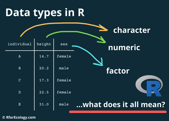
The difference between data types and data structures is that data types refer to the type of data (e.g., numeric, character), while data structures refer to how the data is organized (e.g., vectors, matrices).

Data types

“Most of us are pretty familiar with data types in our daily lives — we can easily tell that things like 1, 2, 3, and 4 are numbers (in this case, integers). 15.7 is still a number, but has a decimal. We know that every single word I’m typing in this sentence is composed of characters, and we know that in math, “true” and “false” are the answers to logical statements.

Just as we do in our heads, R also categorizes our data into different classes. These categories are similar to the real-life ones I described above, but can be a little different in terms of syntax and things to watch out for in your code.”

Selina Cheng

R has several basic data types that you’ll use frequently:

Numeric: For real numbers (decimal and whole). These are useful for calculations and measurements. Read more here
show R code
```
x <- 10.5
class(x)  # "numeric"
```
Integer: Specifically for whole numbers. These are useful for counting and indexing.
show R code
```
y <- 10L  # The 'L' suffix denotes an integer
class(y)  # "integer"
```
Character: For text strings. These are useful for labels and descriptions.
show R code
```
name <- "Dolphin"
class(name)  # "character"
```
Logical: For TRUE/FALSE values. These are useful for conditional statements and logical operations. Read more here
show R code
```
is_mammal <- TRUE
class(is_mammal)  # "logical"
```
Factor: For categorical variables. These are useful for statistical modeling and plotting. They differ from Characters in that they have levels- in other words a fixed set of possible values. read more here
show R code
```
ocean_zones <- factor(c("epipelagic", "mesopelagic", "bathypelagic"))
class(ocean_zones)  # "factor"
```
Complex: For complex numbers. These are useful, eg for signal processing or solving equations.
show R code
```
z <- 1 + 2i
class(z)  # "complex"
```
Raw: For storing raw bytes. These are useful, eg for reading binary files or working with network protocols.
show R code
```
raw_data <- charToRaw("Hello")
class(raw_data)  # "raw"
```

Date and Time: For date and time values. these are useful for time series analysis and plotting.

show R code

current_date <- Sys.Date()
current_time <- Sys.time()
class(current_date)  # "Date"
class(current_time)  # "POSIXct" "POSIXt"

Data Structures

R offers various data structures to efficiently organize and manipulate data:

Indexing

All of these data structures can be indexed. Indexing refers to the method of accessing elements within data structures, such as vectors, matrices, arrays, data frames, and lists. It is a fundamental concept that allows users to efficiently retrieve, modify, and manipulate specific elements within these structures. Indexing is crucial for data analysis and manipulation because it enables precise control over data, allowing for operations like subsetting, filtering, and aggregation. In R, indexing typically starts at 1, which aligns with statistical conventions and makes it intuitive for users familiar with mathematical notation. This is different from many other programming languages that use 0-based indexing. Understanding indexing is essential for writing efficient R code, as it directly impacts the performance and readability of data operations.

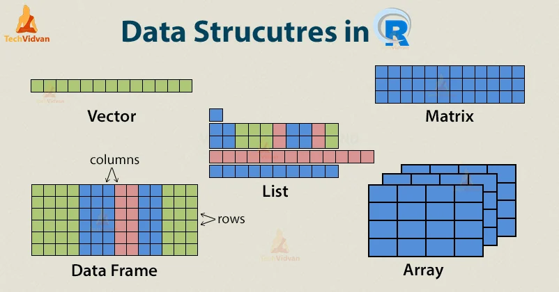
Common Data Structures

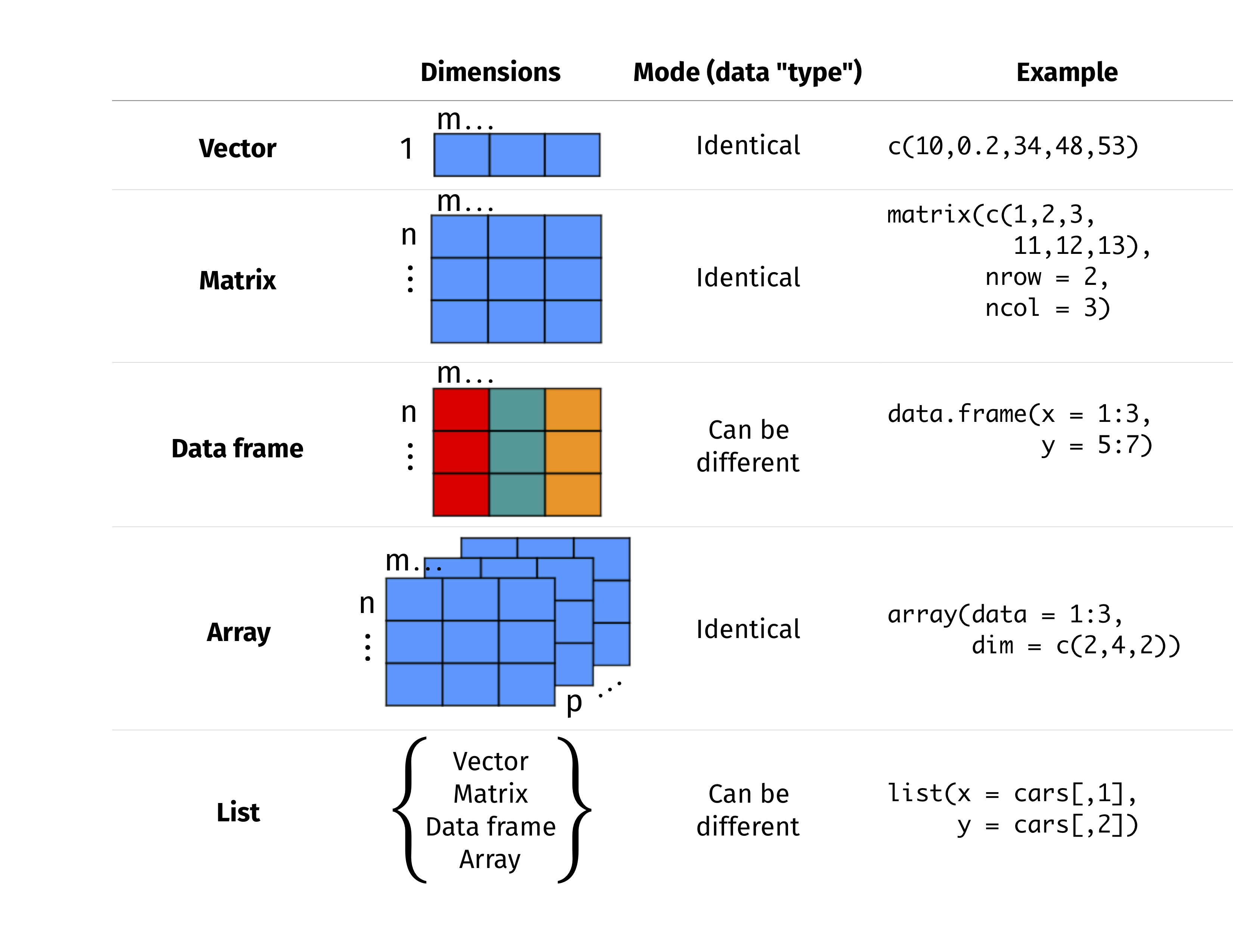
Vectors: One-dimensional arrays holding elements of the same type. These are the most basic data structure in R.

show R code

numeric_vector <- c(1, 2, 3, 4, 5)
character_vector <- c("red", "blue", "green")

# Indexing: Use square brackets
numeric_vector[2]  # 2
numeric_vector[c(1, 3, 5)]  # 1 3 5

Matrices: Two-dimensional arrays holding elements of the same type. These are useful for linear algebra operations.

show R code

m <- matrix(1:6, nrow = 2, ncol = 3)

# Indexing: Use [row, column]
m[1, 2]  # 3
m[, 2]  # 3 4 (entire second column)

Arrays: Multi-dimensional structures holding elements of the same type. These are useful for working with data in more than two dimensions.
show R code
```
arr <- array(1:24, dim = c(2, 3, 4))

# Indexing: Use [dim1, dim2, dim3, ...]
arr[1, 2, 3]  # 13
arr[, , 2]  # 2D slice of the array
```
Data Frames: Table-like structures that can hold different types of data. These are commonly used in data analysis. We will use these most commonly, along with tibbles, which are another version of data frames.
show R code
```
df <- data.frame(
  id = 1:3,
  name = c("Alice", "Bob", "Charlie"),
  score = c(85, 92, 78)
)

# Indexing: Use $ for columns, [row, column] for elements
df$name  # "Alice" "Bob" "Charlie"
df[2, "score"]  # 92
df[df$score > 80, ]  # Rows where score > 80
```
Data frames are particularly useful for handling tabular data. They allow for easy subsetting, merging, and applying functions across columns or rows. Each column can be of a different data type, making them versatile for real-world datasets.

Lists: Can contain elements of different types, including other lists

show R code

my_list <- list(
  numbers = 1:3,
  text = "Hello",
  dataframe = data.frame(x = 1:2, y = c("A", "B"))
)

# Indexing: Use [[]] for single elements, $ for named elements
my_list[[1]]  # 1 2 3
my_list$text  # "Hello"
my_list[["dataframe"]]$x  # 1 2