aov(response_variable ~ factor_1 + factor_2, data = dataset)Introduction to Multi-way ANOVA
In real-world research, we often encounter scenarios where we need to investigate the effects of multiple factors simultaneously. This is where Multi-way ANOVA comes into play. When dealing with two factors, it’s referred to as Two-way ANOVA. This powerful tool allows researchers to not only understand the main effects of each factor but also if there’s an interaction between them, meaning the effect of one factor depends on the level of the other.
Syntax
The syntax for fitting a multi-way ANOVA model in R is similar to that of a one-way ANOVA, with more things on the right side of the ~ operator.
The simplest form of a two-way ANOVA model in R is:
the above code will fit a two-way ANOVA model with response_variable as the dependent variable and factor_1 and factor_2 as the two independent variables. However, this model is missing something important - the interaction term.
aov(response_variable ~ factor_1 + factor_2 + factor_1:factor_2, data = dataset)the above code will fit a two-way ANOVA model with response_variable as the dependent variable and factor_1 and factor_2 as the two independent variables. The factor_1:factor_2 term is the interaction term, which captures the combined effect of both factors on the dependent variable.
this can be simplified as:
aov(response_variable ~ factor_1 * factor_2, data = dataset)above, the * operator is a shorthand for including both main effects and the interaction term in the model.
Interaction Effects
If someone asks you, “Do you prefer ketchup or chocolate sauce on your food?” Undoubtedly, you will respond, “It depends on the type of food!” That’s the “it depends” nature of an interaction effect.
Interaction effects occur when the influence of one factor on the dependent variable is different across the levels of another factor.
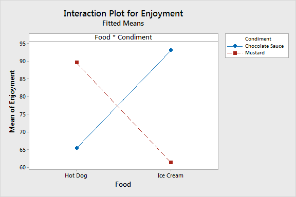
In the plot above, the enjoyment of different condiments is influenced by the type of food they are paired with. For example, while ketchup is preferred with fries, mustard is preferred with hot dogs. This is an interaction effect between the type of condiment and the type of food.
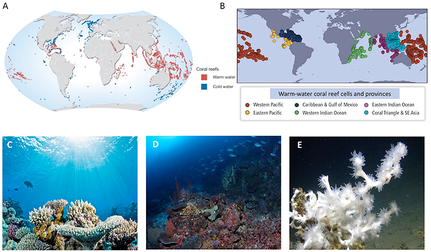
Let’s consider a more relevant example where we’re studying the effect of light and nutrients on coral growth. An interaction would imply that the impact of light on growth isn’t consistent and varies at different nutrient levels. In simpler terms, the effect of one variable (light) changes depending on the level of the other variable (nutrients). Understanding these interactions allows us to unravel the nuanced effects and relationships between different experimental factors.
Interaction Example 1: Different Magnitude of Significance
Let’s navigate through a simulated example exploring the growth of a marine organism under different temperature and nutrient conditions. We’ll simulate growth_data to show an interaction effect where the influence of temperature on growth is different at various nutrient levels.
show R code
# R code for Simulating Data with Interaction Effect
set.seed(42)  # For reproducibility

# Simulating data
growth_data <-
  data.frame(Temperature = rep(c("Low", "High"), each = 50),
             Nutrient = rep(c("Poor", "Rich"), times = 50))

# Adding a response variable with interaction
growth_data$Growth <- with(growth_data,
                           ifelse(
                             Temperature == "Low" & Nutrient == "Poor",
                             rnorm(50, mean = 20, sd = 5),
                             ifelse(
                               Temperature == "High" &
                                 Nutrient == "Poor",
                               rnorm(50, mean = 25, sd = 5),
                               ifelse(
                                 Temperature == "Low" & Nutrient == "Rich",
                                 rnorm(50, mean = 30, sd = 5),
                                 rnorm(50, mean = 40, sd =
                                         5)
                               )
                             )
                           ))
Then, we fit a two-way ANOVA:
# Fitting a two-way ANOVA model
anova_model <-
  aov(Growth ~ Temperature * Nutrient, data = growth_data)

summary(anova_model)
Df Sum Sq Mean Sq F value Pr(>F)
Temperature 1 1348 1348 46.904 7.08e-10 ***
Nutrient 1 3730 3730 129.823 < 2e-16 ***
Temperature:Nutrient 1 166 166 5.761 0.0183 *
Residuals 96 2758 29
---
Signif. codes: 0 '***' 0.001 '**' 0.01 '*' 0.05 '.' 0.1 ' ' 1Here, the growth data is influenced by both temperature and nutrient conditions, and crucially, the effect of temperature on growth changes depending on the nutrient level, showcasing an interaction.
Visualizing and Interpreting Interaction Effects in R
Visual interpretation of interaction effects enhances understanding and communication of findings in scientific studies.
show R code
# Visualizing interaction effects
library(ggplot2)
interaction_plot <-
  ggplot(growth_data, aes(x = Temperature, y = Growth, color = Nutrient)) +
  geom_point(position = position_jitter(width = 0.2), alpha = 0.6) +  # Jitter points to reduce overplotting
  stat_summary(fun = mean,
               geom = "line",
               aes(group = Nutrient),
               size = 1.2) +  # Mean lines for each nutrient level
  labs(
    title = "Interaction Effect of Temperature and Nutrient on Growth",
    y = "Growth",
    x = "Temperature",
    color = "Nutrient Level"
  ) +
  theme_minimal()

interaction_plot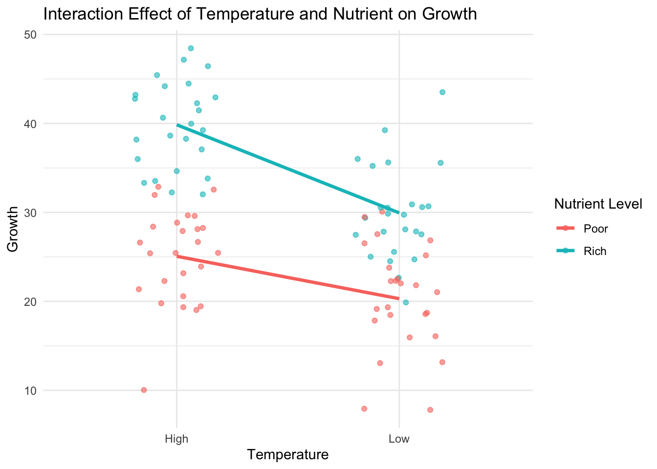
The non-parallel lines in the interaction plot visually depict an interaction between temperature and nutrient conditions, suggesting a more pronounced increase in growth with increased temperature under rich nutrient conditions compared to poor nutrient conditions.
Interaction Example 2: One Significant, One Not Significant
Imagine a slightly different experiment with our marine organism. We might observe a scenario where: - The effect of temperature (Low vs. High) on growth is significant. - The effect of nutrient levels (Poor vs. Rich) is not significant. - There is a significant interaction between temperature and nutrient level.
We’ll simulate growth_data_2:
show R code
# R code for Simulating Data with Specific Interaction Effect
set.seed(90)  # For reproducibility

# Simulating data
growth_data_2 <- data.frame(Temperature = rep(c("Low", "High"), each = 50),
                            Nutrient = rep(c("Poor", "Rich"), times = 50))

# Adding a response variable with interaction
growth_data_2$Growth <- with(growth_data_2,
                             ifelse(
                               Temperature == "High" & Nutrient == "Rich",
                               rnorm(25, mean = 40, sd = 8),
                               ifelse(
                                 Temperature == "Low" &
                                   Nutrient == "Rich",
                                 rnorm(25, mean = 10, sd = 8),
                                 rnorm(50, mean = 25, sd = 8)
                               )
                             ))
And then fit a two-way ANOVA:
# Fitting a two-way ANOVA model
anova_model_2 <-
  aov(Growth ~ Temperature * Nutrient, data = growth_data_2)
summary(anova_model_2)
Df Sum Sq Mean Sq F value Pr(>F)
Temperature 1 6054 6054 97.84 2.54e-16 ***
Nutrient 1 88 88 1.43 0.235
Temperature:Nutrient 1 6054 6054 97.84 2.54e-16 ***
Residuals 96 5940 62
---
Signif. codes: 0 '***' 0.001 '**' 0.01 '*' 0.05 '.' 0.1 ' ' 1In this scenario, despite temperature showing no significant effect on growth, the nutrient level does exhibit a significant effect. Moreover, their interaction also impacts growth.
Visualization and Interpretation
show R code
# Visualizing interaction effects
interaction_plot_2 <-
  ggplot(growth_data_2, aes(x = Temperature, y = Growth, color = Nutrient)) +
  geom_point(position = position_jitter(width = 0.2), alpha = 0.6) +  # Jitter points to reduce overplotting
  stat_summary(fun = mean,
               geom = "line",
               aes(group = Nutrient),
               size = 1.2) +  # Mean lines for each nutrient level
  labs(
    title = "Interaction Effect of Temperature and Nutrient on Growth",
    y = "Growth",
    x = "Temperature",
    color = "Nutrient Level"
  ) +
  theme_minimal()

print(interaction_plot_2)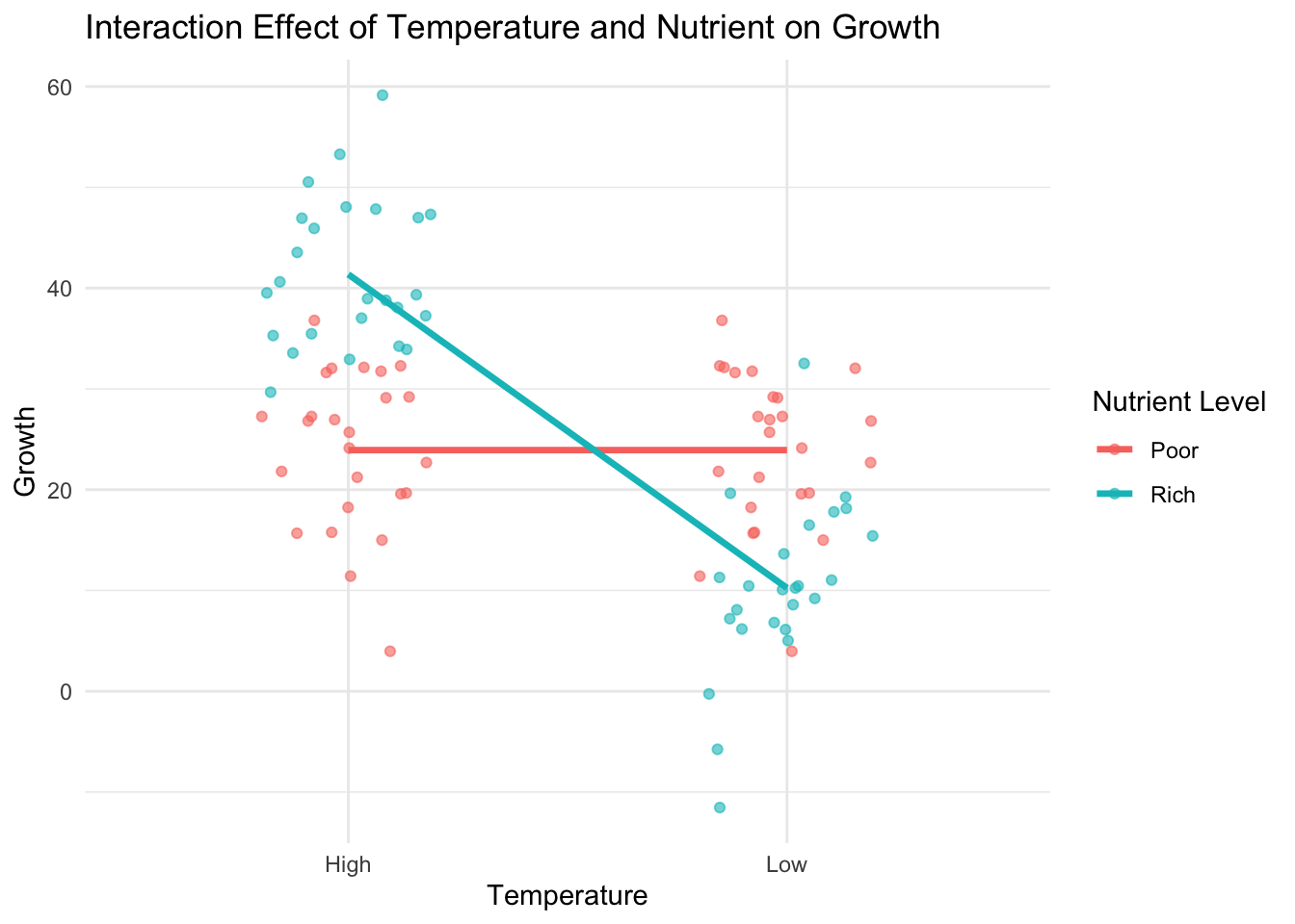
In this plot, while the main effect of temperature might not be statistically significant, the interaction effect suggests that the impact of temperature on growth is different at distinct nutrient levels.
Interaction Example 3: Significance in Opposite Directions
Consider another scenario in our marine organism experiment. This time, the interaction between temperature and nutrient level demonstrates an opposite effect on growth, visually forming an “X” shape in the interaction plot.
show R code
# R code for Simulating Data with Opposite Interaction Effect
set.seed(42)  # For reproducibility

# Simulating data
growth_data_3 <- data.frame(Temperature = rep(c("Low", "High"), each = 50),
                            Nutrient = rep(c("Poor", "Rich"), times = 50))

# Adding a response variable with interaction
growth_data_3$Growth <- with(growth_data_3,
                             ifelse(
                               Temperature == "Low" & Nutrient == "Poor",
                               rnorm(25, mean = 35, sd = 5),
                               ifelse(
                                 Temperature == "High" &
                                   Nutrient == "Poor",
                                 rnorm(25, mean = 25, sd = 5),
                                 ifelse(
                                   Temperature == "Low" & Nutrient == "Rich",
                                   rnorm(25, mean = 25, sd = 5),
                                   rnorm(25, mean = 35, sd =
                                           5)
                                 )
                               )
                             ))
# Fitting a two-way ANOVA model
anova_model_3 <-
aov(Growth ~ Temperature * Nutrient, data = growth_data_3)
summary(anova_model_3) Df Sum Sq Mean Sq F value Pr(>F)
Temperature 1 44.0 44.0 1.619 0.206
Nutrient 1 11.6 11.6 0.428 0.515
Temperature:Nutrient 1 2973.4 2973.4 109.458 <2e-16 ***
Residuals 96 2607.8 27.2
---
Signif. codes: 0 '***' 0.001 '**' 0.01 '*' 0.05 '.' 0.1 ' ' 1This simulated dataset should exhibit an opposite interaction effect, where the effect of one factor reverses across the levels of the second factor.
Visualizing and Understanding Opposite Interactions
show R code
# Visualizing interaction effects
interaction_plot_3 <-
  ggplot(growth_data_3, aes(x = Temperature, y = Growth, color = Nutrient)) +
  geom_point(position = position_jitter(width = 0.2), alpha = 0.6) +  # Jitter points to reduce overplotting
  stat_summary(fun = mean,
               geom = "line",
               aes(group = Nutrient),
               size = 1.2) +  # Mean lines for each nutrient level
  labs(
    title = "Opposite Interaction Effect of Temperature and Nutrient on Growth",
    y = "Growth",
    x = "Temperature",
    color = "Nutrient Level"
  ) +
  theme_minimal()

print(interaction_plot_3)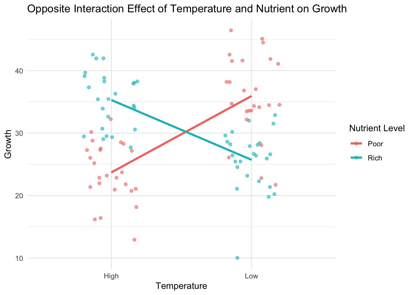
In the interaction plot, you should witness an “X” shape formed by the lines representing each nutrient level, indicating an opposite interaction effect. This implies that while one factor increases the dependent variable under one level of the second factor, it decreases it under the other level.
Hoegh-Guldberg, Ove, Elvira S. Poloczanska, William Skirving, and Sophie Dove. 2017. “Coral Reef Ecosystems Under Climate Change and Ocean Acidification.” Frontiers in Marine Science 4 (May). https://doi.org/10.3389/fmars.2017.00158.