Introduction to the Tidyverse

(moved from last week)

Companion Script

Unfold this code to find a companion script

show R code

# ========================================
# Comprehensive Introduction to the Tidyverse Companion Script
# ========================================

# The Tidyverse is a collection of R packages designed to make data science faster, easier, and more fun.
# It provides a consistent and intuitive framework for data manipulation, visualization, and analysis.

# ----------------------------------------
# Installing and Loading Tidyverse
# ----------------------------------------

# Install Tidyverse (you only need to do this once)
# Uncomment the line below if you haven't installed Tidyverse yet
# install.packages("tidyverse")

# Load Tidyverse (do this every time you start a new R session and want to use Tidyverse)
library(tidyverse)

# ----------------------------------------
# Examples of Tidyverse Functions
# ----------------------------------------

# lets do a quick example (note : BMIs are sort of obsolete and bad science)

# Create a sample dataset
data <- data.frame(
  name = c("Alice", "Bob", "Charlie", "David"),
  sex = c("F", "M", "M", "M"),
  age = c(25, 30, 35, 40),
  height = c(160, 170, 180, 190),
  weight = c(50, 60, 80, 100)
)

# Display the data
head(data)

# 1. filter(): Subset rows based on conditions
data_filtered <- filter(data, sex == "M")
print("Filtered data (males only):")
print(data_filtered)

# 2. select(): Pick columns by name
data_selected <- select(data_filtered, name, age, height, weight)
data_selected <- select(data_filtered, -sex)

print("Selected columns:")
print(data_selected)

# 3. arrange(): Change the order of rows
data_arranged <- arrange(data_selected, desc(age))
print("Arranged data (by age, descending):")
print(data_arranged)

# 4. mutate(): Add new variables
data_mutated <- mutate(data_arranged, bmi = weight / (height/100)^2)
print("Data with BMI added:")
print(data_mutated)

# 5. mutate() with case_when(): Add conditional variables
data_remutated <- mutate(data_mutated, bmi_category = case_when(
  bmi < 18.5 ~ "Underweight",
  bmi < 25 ~ "Normal",
  bmi < 30 ~ "Overweight",
  TRUE ~ "Obese"))
print("Data with BMI category added:")
print(data_remutated)

# Multiple Choice Q2: Which Tidyverse function would you use to create a new column in your dataset?
# a) select()
# b) filter()
# c) mutate()
# d) arrange()

# ----------------------------------------
# The Pipe Operator
# ----------------------------------------

# %>% 
# |>

# The pipe operator (|>) allows you to chain operations together in a more readable way.
# It takes the output of one function and passes it as the first argument to the next function.

# Same operations as above, but using pipes
result_with_pipes <- data |>
  filter(sex == "M") |>
  select(-sex) |>
  arrange(desc(age)) |>
  mutate(
    bmi = weight / (height/100)^2,
    bmi_category = case_when(
      bmi < 18.5 ~ "Underweight",
      bmi < 25 ~ "Normal",
      bmi < 30 ~ "Overweight",
      TRUE ~ "Obese"
    )
  )

result_with_pipes

# Multiple Choice Q3: What does the pipe operator (|>) do in R?
# a) It creates a new variable
# b) It filters the data
# c) It passes the output of one function as the input to the next function
# d) It arranges the data in descending order

# ----------------------------------------
# Key Tidyverse Packages
# ----------------------------------------

# 1. dplyr: For data manipulation
# 2. tidyr: For tidying data
# 3. ggplot2: For data visualization
# 4. readr: For reading rectangular data
# 5. purrr: For functional programming
# 6. tibble: For modern data frames

# ----------------------------------------
# Data Transformation with dplyr
# ----------------------------------------

# Let's use a real dataset for this example
fish_data <- read.csv("https://raw.githubusercontent.com/laurenkolinger/MES503data/main/week3/s4pt4_fishbiodivCounts_23sites_2014_2015.csv")

fish_summary <- fish_data |>
  filter(year == 2015) |>
  group_by(trophicgroup) |>
  summarise(
    avg_count = mean(counts),
    total_count = sum(counts)
  ) |>
  arrange(desc(total_count))

print("Summary of fish data:")
print(fish_summary)

# Multiple Choice Q5: In the code above, what does the group_by() function do?
# a) It filters the data for specific groups
# b) It arranges the data by group
# c) It creates separate groups for subsequent operations
# d) It counts the number of groups in the data

# ----------------------------------------
# Data Visualization with ggplot2
# ----------------------------------------

# Basic structure of a ggplot:
# ggplot(data = <DATA>) +
#   <GEOM_FUNCTION>(mapping = aes(<MAPPINGS>))

# Create a boxplot of fish counts by trophic group
ggplot(fish_data, aes(x = trophicgroup, y = counts)) +
  geom_boxplot() +
  theme_minimal() +
  labs(title = "Fish Counts by Trophic Group",
       x = "Trophic Group",
       y = "Count")

# Multiple Choice Q6: In ggplot2, what does the aes() function do?
# a) It adds aesthetic elements like colors and shapes to the plot
# b) It specifies the axes of the plot
# c) It maps variables in the data to visual properties of the plot
# d) It arranges multiple plots in a grid

# ----------------------------------------
# Practice Script: Lab Assignment 1 in R
# ----------------------------------------

# Load required libraries
library(readxl)
library(dplyr)
library(ggplot2)
library(httr)

# Download Excel file from GitHub and read it
url <- "https://github.com/laurenkolinger/MES503data/raw/main/week1/TCRMP-RAPID-Dec2017-Health-intercept.xlsx"
temp_file <- tempfile(fileext = ".xlsx")
GET(url, write_disk(temp_file))
dat <- read_excel(temp_file, sheet = "DATA")

# Create a summary of the length data for specified species
length_summary <- dat |> 
  filter(SPP %in% c("AA", "OA", "OFAV", "OFRA", "PA", "SS")) |>
  group_by(SPP) |>
  summarise(
    mean_length = mean(LENGTH),
    sd_length = sd(LENGTH),
    SEM_length = sd(LENGTH)/sqrt(length(LENGTH))
  )

# Plot the average length of the specified species with error bars
ggplot(length_summary, aes(x=SPP, y=mean_length)) +
  geom_bar(stat="identity") +
  geom_errorbar(aes(ymin = mean_length-SEM_length, ymax = mean_length+SEM_length), width = 0.2) +
  xlab("species") +
  ylab("length (cm)") +
  ggtitle("average length of 6 common coral species ± SEM")

# Create a summary of the count and percentage of observations for each transect and species
prev_summary <- dat |> 
  group_by(TRANSECT, SPP) |>
  summarise(count = n()) |>
  mutate(percentage = (count/sum(count))*100) |>
  filter(SPP=="MC")

print("Prevalence summary:")
print(prev_summary)

As you’ve been working with R, you may have noticed that some tasks can become quite complex, requiring multiple steps and creating intermediate variables. This is where the Tidyverse comes in - a collection of R packages designed to make data science faster, easier, and more fun. Let’s dive into this powerful toolkit, starting with one of its most revolutionary features: the pipe operator.

Install Tidyverse

you only need to do this once.

install.packages("tidyverse")

This will load several other packages, including dplyr, ggplot2, and tibble, among many others.

Load Tidyverse

Do this any time you need to use any of thes packages above. This is faster than loading single packages, but also common to see single packages loaded (e.g., library(ggplot2) ).

library(tidyverse)

Some examples of Tidyverse functions

lets say we have some data

data <- data.frame(
  name = c("Alice", "Bob", "Charlie", "David"),
  sex = c("F", "M", "M", "M"),
  age = c(25, 30, 35, 40),
  height = c(160, 170, 180, 190),
  weight = c(50, 60, 80, 100)
)
head(data)

     name sex age height weight
1   Alice   F  25    160     50
2     Bob   M  30    170     60
3 Charlie   M  35    180     80
4   David   M  40    190    100

lets filter the data to include only Males

data_filtered <- filter(data, sex == "M")

head(data_filtered)

     name sex age height weight
1     Bob   M  30    170     60
2 Charlie   M  35    180     80
3   David   M  40    190    100

lets select all but the sex column

#either keep all the columns you want
data_selected <- select(data_filtered, name, age, height, weight)

#or remove the column you dont. 
data_selected <- select(data_filtered, -sex)

head(data_selected)

     name age height weight
1     Bob  30    170     60
2 Charlie  35    180     80
3   David  40    190    100

lets arrange the data by age in descending order (from oldst to youngest)

data_arranged <- arrange(data_selected, desc(age))

head(data_arranged)

     name age height weight
1   David  40    190    100
2 Charlie  35    180     80
3     Bob  30    170     60

lets make a new column bmi by mutating the data BMI = weight (kg) / height (m)²

data_mutated <- mutate(data_arranged, bmi = weight / (height/100)^2)

head(data_mutated)

     name age height weight      bmi
1   David  40    190    100 27.70083
2 Charlie  35    180     80 24.69136
3     Bob  30    170     60 20.76125

lets make another new column bmi_category by mutating the data again

data_remutated <- mutate(data_mutated, bmi_category = case_when(
  bmi < 18.5 ~ "Underweight",
  bmi < 25 ~ "Normal",
  bmi < 30 ~ "Overweight",
  TRUE ~ "Obese"))

head(data_remutated)

     name age height weight      bmi bmi_category
1   David  40    190    100 27.70083   Overweight
2 Charlie  35    180     80 24.69136       Normal
3     Bob  30    170     60 20.76125       Normal

nice! there are tons of other functions in the tidyverse, but this is just a sampling of some of the handy ones.

Though this is handy,there is still an even better way to do this using the same functions.

data_remutated <- data |>
  filter(sex == "M") |>
  select(-sex) |>
  arrange(desc(age)) |>
  mutate(bmi = weight / (height/100)^2) |>
  mutate(bmi_category = case_when(
    bmi < 18.5 ~ "Underweight",
    bmi < 25 ~ "Normal",
    bmi < 30 ~ "Overweight",
    TRUE ~ "Obese"))

data_remutated

     name age height weight      bmi bmi_category
1   David  40    190    100 27.70083   Overweight
2 Charlie  35    180     80 24.69136       Normal
3     Bob  30    170     60 20.76125       Normal

The notation above `|>`` is called the pipe operator. It allows you to chain operations together in a more readable way. Lets learn more here:

The Pipe Operator

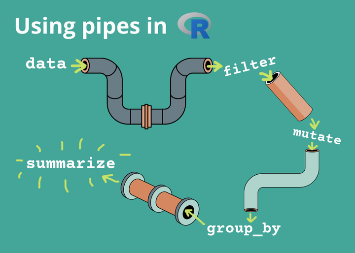
The pipe operator |> (or %>% in older R versions) is a key feature of the tidyverse. It allows you to chain operations in a readable way.

The pipe takes the output of one function and passes it as the first argument to the next function.

Imagine you’re in a kitchen, preparing a meal. You need to wash, chop, and cook your ingredients. In traditional R, you might do something like this:

ingredients <- c("carrot", "potato", "onion")
washed <- wash(ingredients)
chopped <- chop(washed)
cooked <- cook(chopped)

# another way of putting this:
cooked <- cook(chop(wash(ingredients)))

This works, but it’s not very intuitive. You have to read from the inside out, and you’re creating multiple intermediate variables. Now, let’s see how the pipe operator (|> or %>%) changes this:

ingredients <- c("carrot", "potato", "onion")
meal <- ingredients |>
  wash() |>
  chop() |>
  cook()

See how much more readable that is? It’s like a recipe: take the ingredients, then wash them, then chop them, then cook them. The pipe takes the output of one function and feeds it as the input to the next function.

Why the Pipe Works

The pipe operator works by taking the output of the expression on its left and passing it as the first argument to the function on its right. It’s as if each function is saying, “Give me what you’ve got so far, and I’ll do my part.”

This approach has several benefits: 1. It makes your code more readable and intuitive. 2. It reduces the need for intermediate variables. 3. It allows you to think about your data in a step-by-step manner.

Pipes vs. Regular Function Calls

Let’s compare pipes to regular function calls using a real data example. We’ll use the mtcars dataset, which is built into R.

Regular function calls:

data(mtcars)
sorted_data <- arrange(mtcars, mpg)
filtered_data <- filter(sorted_data, cyl == 6)
selected_data <- select(filtered_data, mpg, hp)
final_result <- mutate(selected_data, kpl = mpg * 0.425)
head(final_result)

               mpg  hp    kpl
Merc 280C     17.8 123 7.5650
Valiant       18.1 105 7.6925
Merc 280      19.2 123 8.1600
Ferrari Dino  19.7 175 8.3725
Mazda RX4     21.0 110 8.9250
Mazda RX4 Wag 21.0 110 8.9250

Now, let’s do the same operations using pipes:

library(dplyr)

data(mtcars)
final_result <- mtcars |>
  arrange(mpg) |>
  filter(cyl == 6) |>
  select(mpg, hp) |>
  mutate(kpl = mpg * 0.425)
head(final_result)

               mpg  hp    kpl
Merc 280C     17.8 123 7.5650
Valiant       18.1 105 7.6925
Merc 280      19.2 123 8.1600
Ferrari Dino  19.7 175 8.3725
Mazda RX4     21.0 110 8.9250
Mazda RX4 Wag 21.0 110 8.9250

The piped version is more concise and reads like a series of steps: “Take mtcars, then arrange by mpg, then filter for 6 cylinders, then select mpg and hp, then mutate to add kpl.”

Also note the syntax (wording) used in the Some examples section above. Same thing.

Key Tidyverse Packages

The Tidyverse includes several packages, each designed for specific tasks:

dplyr: For data manipulation
tidyr: For tidying data
ggplot2: For data visualization
readr: For reading rectangular data
purrr: For functional programming
tibble: For modern data frames

Let’s explore some key functions from dplyr and ggplot2.

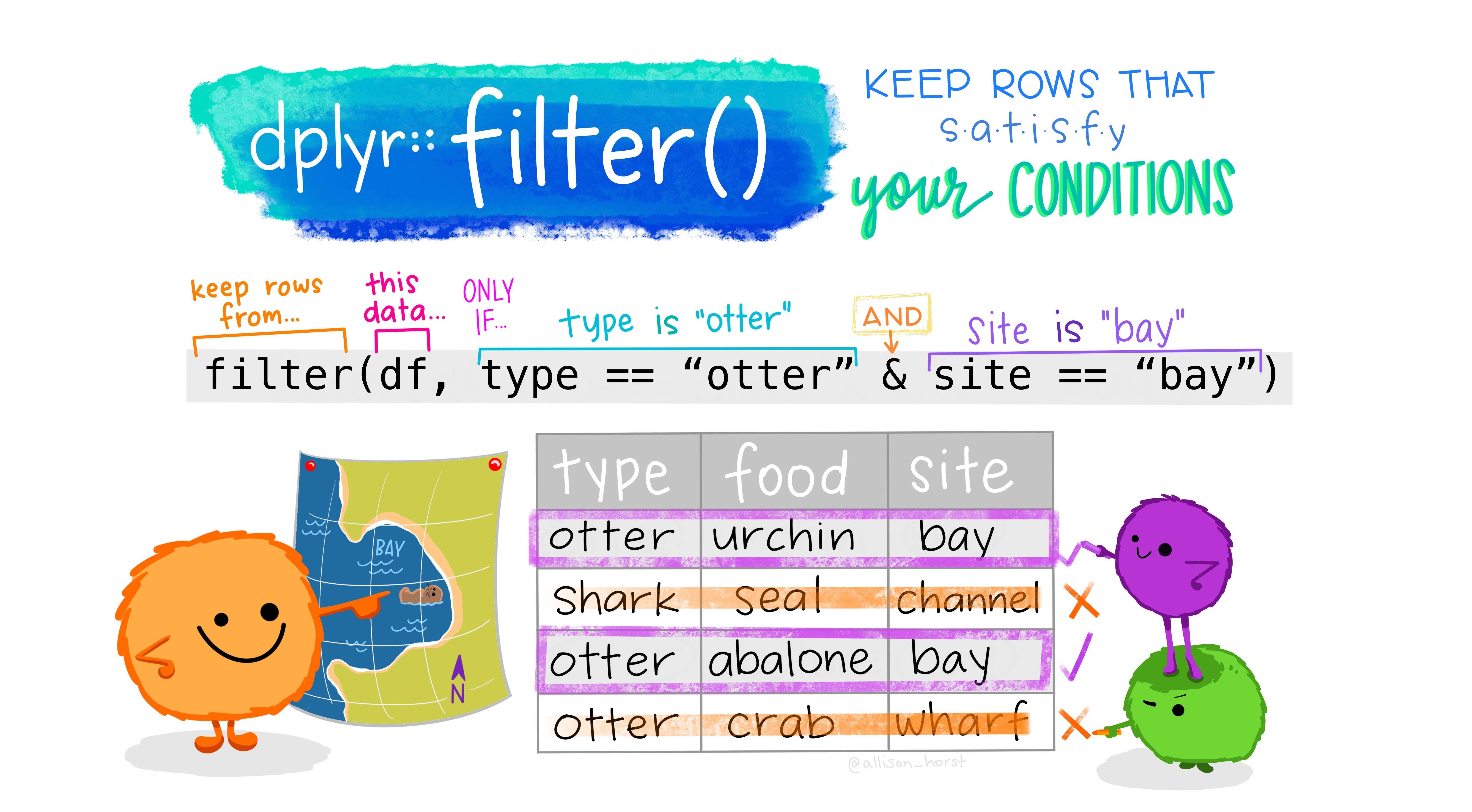
Data Transformation with dplyr

dplyr provides a set of verbs for data manipulation:

filter(): Subset rows based on conditions
select(): Pick columns by name
mutate(): Add new variables
summarise(): Reduce variables to values
arrange(): Change the order of rows

Let’s use these with our fish data:

library(dplyr)

fish_data <- read.csv("https://raw.githubusercontent.com/laurenkolinger/MES503data/main/week3/s4pt4_fishbiodivCounts_23sites_2014_2015.csv")

fish_summary <- fish_data |>
  filter(year == 2015) |>
  group_by(trophicgroup) |>
  summarise(
    avg_count = mean(counts),
    total_count = sum(counts)
  ) |>
  arrange(desc(total_count))

print(fish_summary)

# A tibble: 4 × 3
  trophicgroup avg_count total_count
  <chr>            <dbl>       <int>
1 plank            34.0        30317
2 herb              9.85       19289
3 inv               3.85        8529
4 pisc              2.80        1188

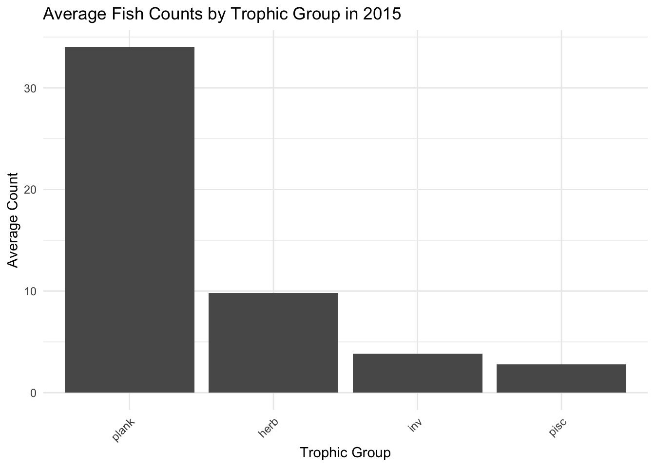
This code filters for 2015 data, groups by trophic group, calculates average and total counts, and arranges the results by total count in descending order.

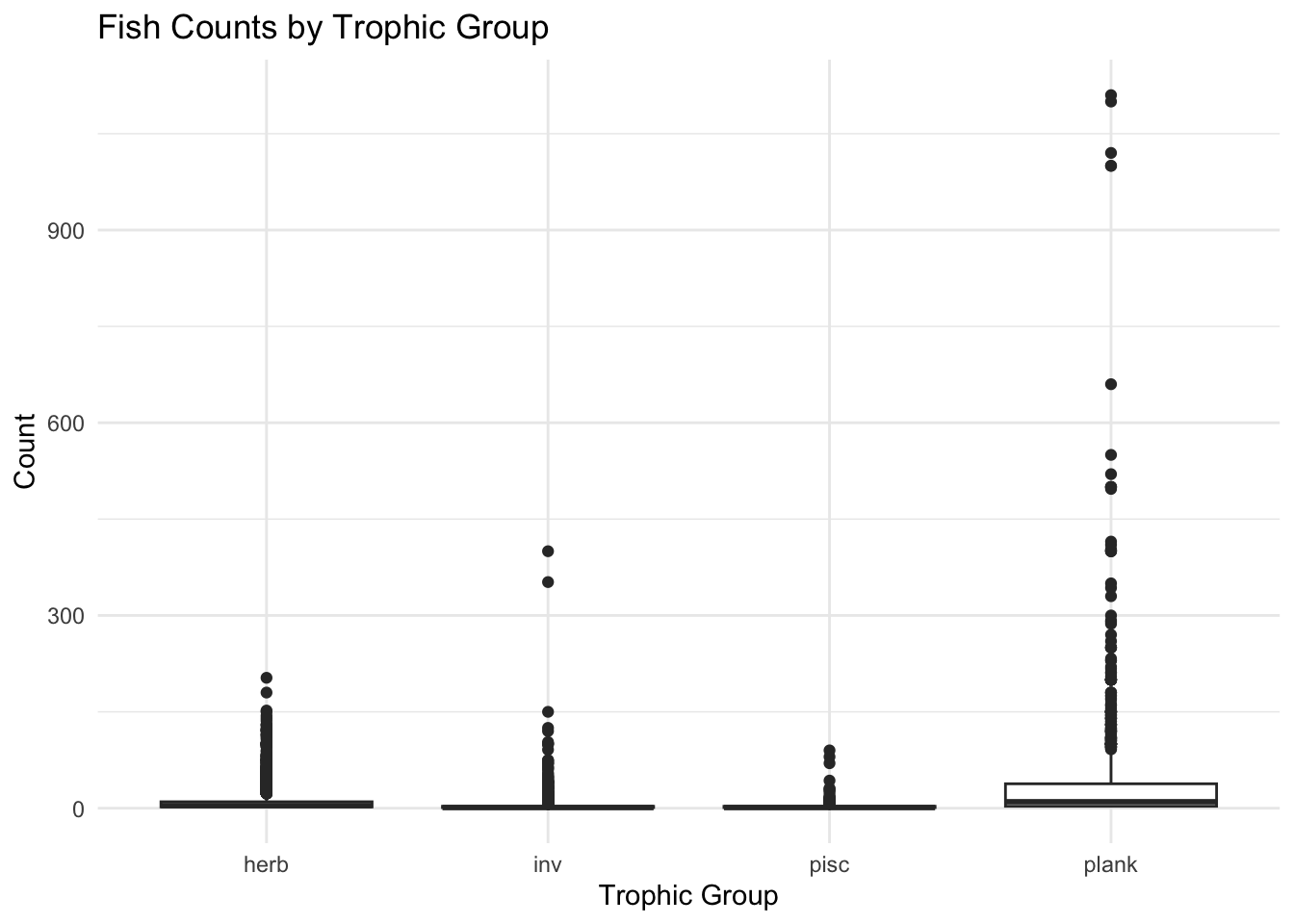
Data Visualization with ggplot2

ggplot2 is based on the Grammar of Graphics, allowing you to build plots layer by layer. Here’s a basic structure:

ggplot(data = <DATA>) +
  <GEOM_FUNCTION>(mapping = aes(<MAPPINGS>))

Let’s create a plot using our fish data:

library(ggplot2)

ggplot(fish_data, aes(x = trophicgroup, y = counts)) +
  geom_boxplot() +
  theme_minimal() +
  labs(title = "Fish Counts by Trophic Group",
       x = "Trophic Group",
       y = "Count")

This creates a boxplot showing the distribution of fish counts for each trophic group.

Putting It All Together

Now, let’s combine data transformation and visualization:

fish_data |>
  filter(year == 2015) |>
  group_by(trophicgroup) |>
  summarise(avg_count = mean(counts)) |>
  ggplot(aes(x = reorder(trophicgroup, -avg_count), y = avg_count)) +
  geom_col() +
  theme_minimal() +
  labs(title = "Average Fish Counts by Trophic Group in 2015",
       x = "Trophic Group",
       y = "Average Count") +
  theme(axis.text.x = element_text(angle = 45, hjust = 1))

This code filters the data, calculates average counts by trophic group, and creates a bar plot of the results.

Practice Script : Lab assignment 1 in R

Copy this into your R script to run the code to complete lab assignment 1 in 18 lines of code

# load libraries 
library(readxl)
library(dplyr)
library(ggplot2)
library(httr)

# download excel file from github and read in as dat
url <- "https://github.com/laurenkolinger/MES503data/raw/main/week1/TCRMP-RAPID-Dec2017-Health-intercept.xlsx"
temp_file <- tempfile(fileext = ".xlsx")
GET(url, write_disk(temp_file))
dat <- read_excel(temp_file, sheet = "DATA")

# Create a summary of the length data for the specified species
length_summary <- dat |> 
  filter(SPP %in% c("AA", "OA", "OFAV", "OFRA", "PA", "SS")) |>  # Filter rows to include only the specified species
  group_by(SPP) |>  # Group data by species
  summarise (
    mean_length = mean(LENGTH),
    sd_length = sd(LENGTH),
    SEM_length = sd(LENGTH)/sqrt(length(LENGTH))
  )  # Compute summary statistics: mean, standard deviation, and standard error of mean for length
print(length_summary)

# Plot the average length of the specified species with error bars
ggplot(length_summary, aes(x=SPP,y=mean_length))+
  geom_bar(stat="identity") +  # Create bars for mean length
  geom_errorbar(aes(ymin = mean_length-SEM_length, ymax = mean_length+SEM_length), width =0.2) +  # Add error bars 
  xlab("species") +    # Label the x-axis
  ylab("length (cm)") +   # Label the y-axis
  ggtitle("average length of 6 common coral species ± SEM")  # Add a title to the plot

# Create a summary of the count and percentage of observations for each transect and species
prev_summary <- dat |> 
  group_by(TRANSECT, SPP) |>   # Group data by transect and species
  summarise(count = n()) |>    # Compute count of observations for each group
  mutate(percentage = (count/sum(count))*100) |>    # Compute the percentage of observations for each group relative to the total count
  filter(SPP=="MC")  # Filter rows to include only the species "MC"

prev_summary