             Df Sum Sq Mean Sq F value Pr(>F)
MPA_Type      2  19869    9935   111.7 <2e-16 ***
Residuals   147  13070      89
---
Signif. codes: 0 '***' 0.001 '**' 0.01 '*' 0.05 '.' 0.1 ' ' 1Performing ANOVA in R and Testing Assumptions
Formatting the data
Before running ANOVA, it’s crucial to ensure the dataset is structured appropriately. For ANOVA, the data is typically in a “long” format, where one column represents the grouping variable (in our case, MPA_Type) and another represents the dependent variable (e.g., fish abundance).
Our data_fish_mpa has columns named MPA_Type (the grouping variable, or main effect, or factor) and Fish_Biomass (the measured variable, aka dependent, or response variable) Each row represents a sample from a specific MPA type with a recorded fish abundance.
review
what are the levels of MPA_Type ?
hint: use unique() to find the unique values in a column
Conducting the ANOVA in R
To perform a one-way ANOVA in R, you can use the aov() function. Here’s the formula for our fish example:
Checking Assumptions
1. Independence:
observations within each group must be independent.
Avoiding “pseudo-replication” (using the same sample more than once) and ensuring proper study design can help maintain the independence of observations.
2. Homogeneity of Variance (Homoscedasticity)
-
Bartlett Test: This test checks for equal variances across groups
\(H_0\) : All groups have the same variance.
\(H_1\) : At least two groups have different variances.
If p > 0.05, This suggests that there’s no significant evidence against the assumption of equal variances across groups. You can proceed with tests like ANOVA that assume equal variances across groups.
If p < 0.05, This suggests that there’s evidence to believe that the variances are not equal across all groups. In the context of ANOVA, this might indicate that the assumption of homoscedasticity is violated.
bartlett.test(Fish_Biomass ~ MPA_Type, data = data_fish_mpa)
    Bartlett test of homogeneity of variances

data:  Fish_Biomass by MPA_Type
Bartlett's K-squared = 1.0967, df = 2, p-value = 0.5779- Another way to test this assumption is with a plot of residuals vs. fitted values, which we learned last week.
3. Normality of residuals:
- Calculate the standardized residuals of the
anova_result model. Standardized residuals are the residuals divided by their estimated standard errors. They help in understanding how many standard deviations a residual is away from the expected value (which is zero for well-fitted data).
aov2.stdres <- rstandard(anova_result)-
The Shapiro-Wilk test is a formal statistical test for the normality of data.
\(H_0\) : data follow a normal distribution.
\(H_1\) : data do not follow a normal distribution
If p > 0.05, you would not reject the null hypothesis, suggesting the data are likely normally distributed, fulfilling this assumption for ANOVA
If p < 0.05, you reject the null hypothesis, indicating that the data does not follow a normal distribution. At this point, you may want to transform your data or try another statistical test.
shapiro.test(aov2.stdres)
    Shapiro-Wilk normality test

data:  aov2.stdres
W = 0.99657, p-value = 0.9813-
Plot a histogram of the standardized residuals (we allso)
- If the histogram looks bell-shaped (like a normal distribution), it’s an indication that this assumption might be met.
hist(aov2.stdres) 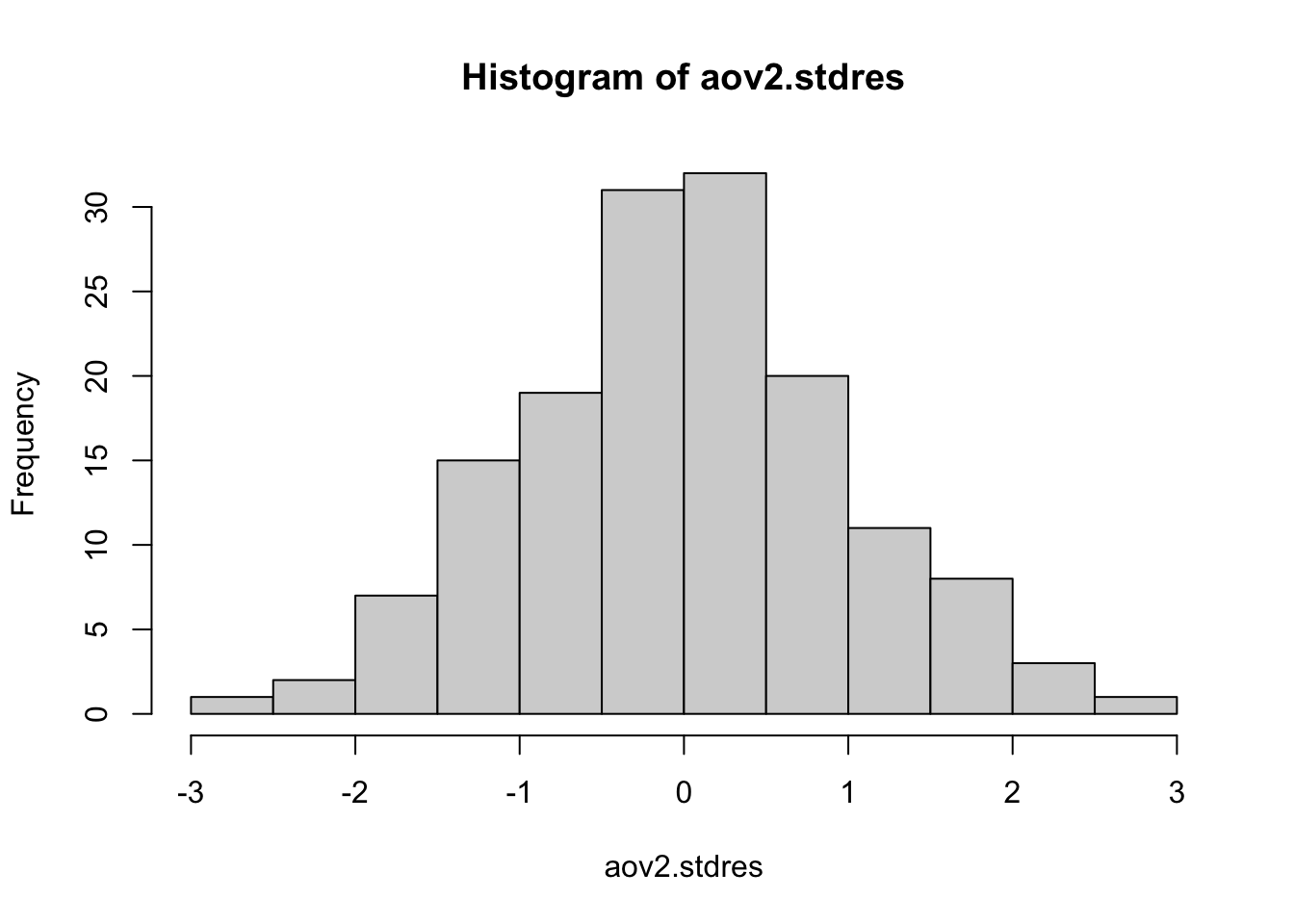
-
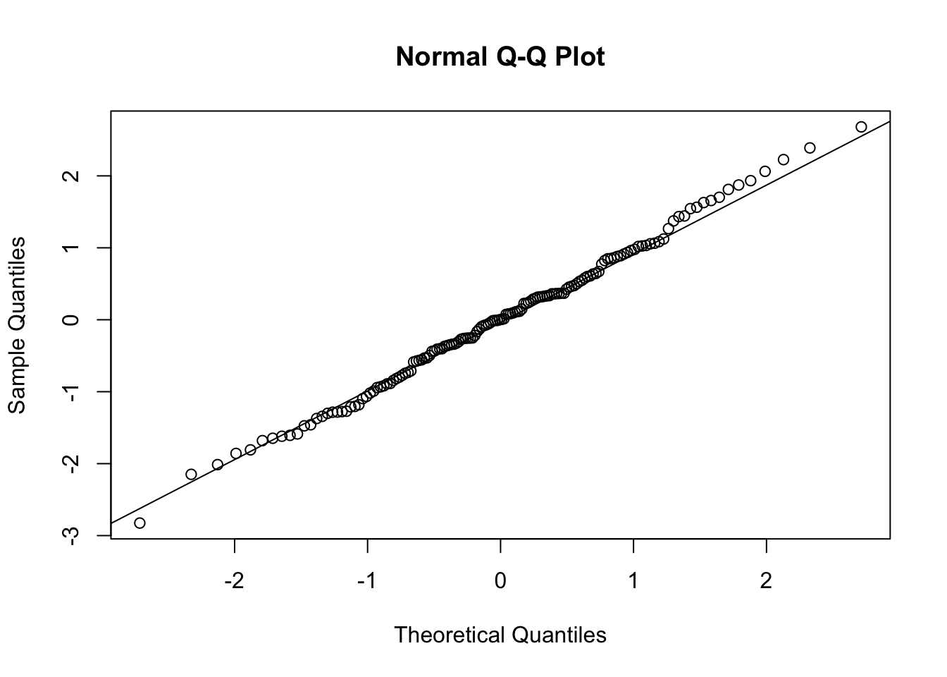
Plot with QQ-plot:
- This line produces a Quantile-Quantile (Q-Q) plot for the standardized residuals.In a Q-Q plot, if the residuals lie on or around the straight line (often called the QQ line), it indicates that the residuals are normally distributed. Deviations from this line can indicate departures from normality.
Can we proceed?
We performed the ANOVA using aov() and tested the three assumptions. We determined that the three assumptions were met. Now we can interpret the results of the aov() output…