Like a one-way ANOVA, we must test multi-way ANOVAs for some assumptions. Let’s illustrate these assumptions with our simulated growth_data_2 (from Section 62).
Assumption 1: Normality
Residuals from the model should exhibit a normal distribution. We can test this using the Shapiro-Wilk test on the standardized residuals.
# Fitting the model using growth_data_2anova_model_2<-aov(Growth~Temperature*Nutrient, data =growth_data_2)summary(anova_model_2)
                     Df Sum Sq Mean Sq F value   Pr(>F)
Temperature           1   6054    6054   97.84 2.54e-16 ***
Nutrient              1     88      88    1.43    0.235
Temperature:Nutrient  1   6054    6054   97.84 2.54e-16 ***
Residuals            96   5940      62
---
Signif. codes:  0 '***' 0.001 '**' 0.01 '*' 0.05 '.' 0.1 ' ' 1
    Shapiro-Wilk normality test

data:  rstandard(anova_model_2)
W = 0.98226, p-value = 0.1987
The Shapiro-Wilk test result (W = 0.98, p-value = 0.2) suggests that the residuals are normally distributed, as the p-value is greater than the standard significance level of 0.05. Therefore, the normality assumption is met.
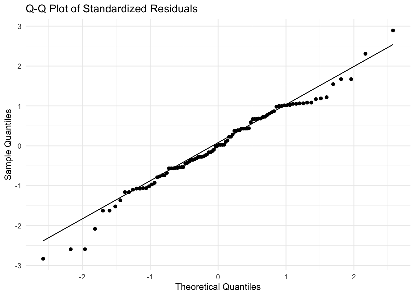
We can also visualize the normality of residuals using a Q-Q plot.
The residuals align closely with the straight line, indicating normality.
Assumption 2: Homogeneity of Variance
The Bartlett test checks if the variances across groups are equal.
For a multi-way ANOVA, it’s not necessary for the Bartlett test to pass each individual factor separately (e.g., for both Temperature and Nutrient), but the overall test of variances should not show significant differences for the interaction between the factors.
IF you tried to run the Bartlett test on the interaction term (Temperature:Nutrient), you would get an error. This is because the bartlett.test function does not support formulas with interactions. Instead, you can create an interaction term manually and then run the Bartlett test.
# This would give you an error# bartlett.test(Growth ~ Temperature*Nutrient, data = growth_data_2)# Create an interaction term for Temperature and Nutrientgrowth_data_2$Temp_Nutrient<-interaction(growth_data_2$Temperature, growth_data_2$Nutrient)# Perform Bartlett's test with the interaction termbartlett.test(Growth~Temp_Nutrient, data =growth_data_2)
    Bartlett test of homogeneity of variances

data:  Growth by Temp_Nutrient
Bartlett's K-squared = 0.76339, df = 3, p-value = 0.8582
If the Bartlett test on the interaction term passes (i.e., no significant difference in variances between the groups), it suggests that the homogeneity of variance assumption is satisfied for the two-way ANOVA.
This Bartlett test result (X-squared = 0.76=, df = 3, p= 0.8582) indicates that the variances are equal across the groups.
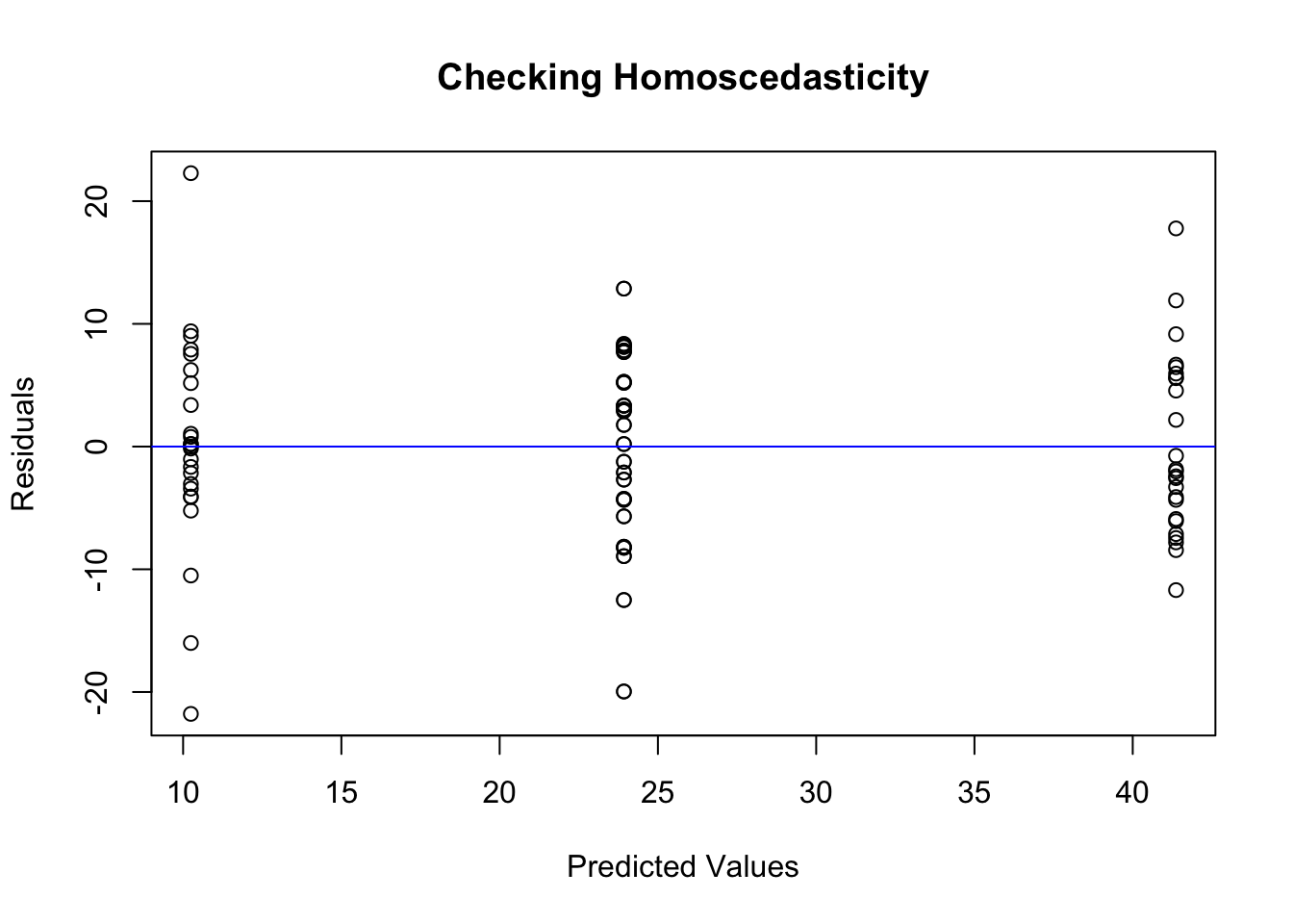
We can also visualize the homogeneity of variance using a residuals vs. fitted values plot.
model<-aov(Growth~Temperature*Nutrient, data =growth_data_2)residuals_data<-residuals(model)predicted_values<-fitted(model)plot(predicted_values, residuals_data, xlab="Predicted Values", ylab="Residuals", main="Checking Homoscedasticity")abline(h=0, col="blue")
In this plot, the residuals are clustered and form a pattern that is typical when there are categorical predictors in the model (in our case, Temperature and Nutrient), leading to discrete predicted values rather than a continuous spread.
This pattern is normal if both Temperature and Nutrient are categorical factors…
… which they are for us. In this case, you can still use this plot to check for trends in the residuals (e.g., increasing variance as predicted values increase),
The Bartlett test is sensitive to deviations from normality. If your data is not normally distributed, a Levene’s test might be a better alternative, as it is less sensitive to non-normality and can still check for homogeneity of variances.
Levene's Test for Homogeneity of Variance (center = median)
      Df F value Pr(>F)
group  3  0.0373 0.9903
      96
The Levene’s test result (F value = 0.0373, Pr(>F) = 0.9903) indicates that the variances are equal across the groups, as the p-value is greater than 0.05. Thus, the homogeneity of variance assumption is satisfied.
Assumption 3: Independent Observations
Ensuring observations are independent and randomly sampled is paramount. This is done during the experimental phase, not during the statistical analysis phase. But it is an essential assumption to prevent spurious errors.
Addressing Violations
If the normality assumption is violated, one can explore transformations or non-parametric alternatives. For homogeneity violations, engaging with robust ANOVA methods or transformations might be helpful. Violations of independence can be addressed by ensuring randomization in the experimental design.
Important note About Assumptions
Statistics, especially when applied to real-world data, isn’t always a rigid process where all assumptions must be perfectly met. Instead, it’s often more flexible and nuanced, especially when it comes to testing assumptions like normality and equal variances. As you begin to explore statistical tests like ANOVA, it’s important to understand that statistics is as much an art as it is a science. Much like a lawyer builds a case in court, a statistician builds an argument for why their results are valid, even when certain assumptions may not be perfectly satisfied.
For ANOVA, two key assumptions are:
Normality: The data in each group should be normally distributed.
Homoscedasticity (equal variances): The variability of data points (the spread or “scatter” of values) should be similar across all groups being compared.
These assumptions help ensure that the F-test used in ANOVA gives accurate results.
However, real-world data is messy, and it’s rare for data to perfectly fit all assumptions. This doesn’t necessarily mean you need to abandon the test; instead, you need to evaluate how much the data deviates from these assumptions and whether those deviations are serious enough to affect your conclusions.
ANOVA’s Robustness to Deviations
ANOVA is considered somewhat robust to moderate deviations from normality, meaning that small departures from a perfectly normal distribution won’t necessarily invalidate the results.
This is especially true when you have a large sample size, because with more data points, the central limit theorem kicks in and the results of ANOVA become more reliable, even if the underlying data isn’t perfectly normal.
However, ANOVA is less tolerant of unequal variances across groups. If the groups you’re comparing have widely different variances, it can lead to biased results and incorrect conclusions. This is why we use tests like Levene’s test to check for homoscedasticity. If the variances are unequal, the ANOVA results might not be reliable, and alternative methods should be considered.
Why Deviations Aren’t Always Dealbreakers
The key takeaway is that not every small deviation from an assumption invalidates your analysis. In fact, statistical tests are tools, and like any tool, their usefulness depends on how and when they are applied. Think of a statistician like a lawyer presenting a case:
The data is the evidence.
The tests are the tools used to examine that evidence.
The conclusion (your results) needs to be supported by a strong argument that the data can be trusted.
For example: - If the Shapiro-Wilk test indicates that your data isn’t perfectly normal, but the data isn’t extremely skewed or oddly shaped, you might proceed with ANOVA—especially if you have a large sample size—and explain in your report that while the normality assumption wasn’t strictly met, the deviation was small enough to not heavily impact the results. - If Levene’s test shows that variances are nearly equal but not perfectly so, you might still proceed with ANOVA, while acknowledging the slight violation and considering a follow-up analysis (like Welch’s ANOVA) to confirm your findings.
Transparency is Key
When assumptions are slightly violated, it’s important to be transparent. Acknowledging and explaining these deviations is crucial. Just as a lawyer presents evidence and then interprets it to argue their case, a statistician must present the results of assumption tests and explain whether and how they affect the final conclusions.
For instance, you could say: > “The Shapiro-Wilk test indicated a small deviation from normality (p = 0.04), but given the large sample size (n = 100) and the near-normal shape of the distribution, the impact on the ANOVA results is likely minimal. Thus, we proceeded with ANOVA while keeping this limitation in mind.”
Statistics is a Craft
Statistics is rarely black and white. Instead, it involves critical thinking and judgment calls. You’re not simply running tests and following their results blindly—you’re building an argument for why your analysis is valid, even when real-world data doesn’t perfectly match the textbook assumptions. Your ability to interpret and present your findings, along with acknowledging limitations and potential biases, is what makes statistics more like a craft or an art form.
So, when conducting an analysis:
Check the assumptions.
Interpret the results of those checks.
Be transparent about any violations and how they affect your conclusions.
If necessary, adjust your analysis or use alternative methods, but understand that not all deviations require drastic changes.
By balancing these factors, you’re essentially acting like a lawyer—presenting the best case for the reliability and objectivity of your data and conclusions. This approach allows you to make sound, well-supported statistical arguments even when things aren’t perfect.