Activity

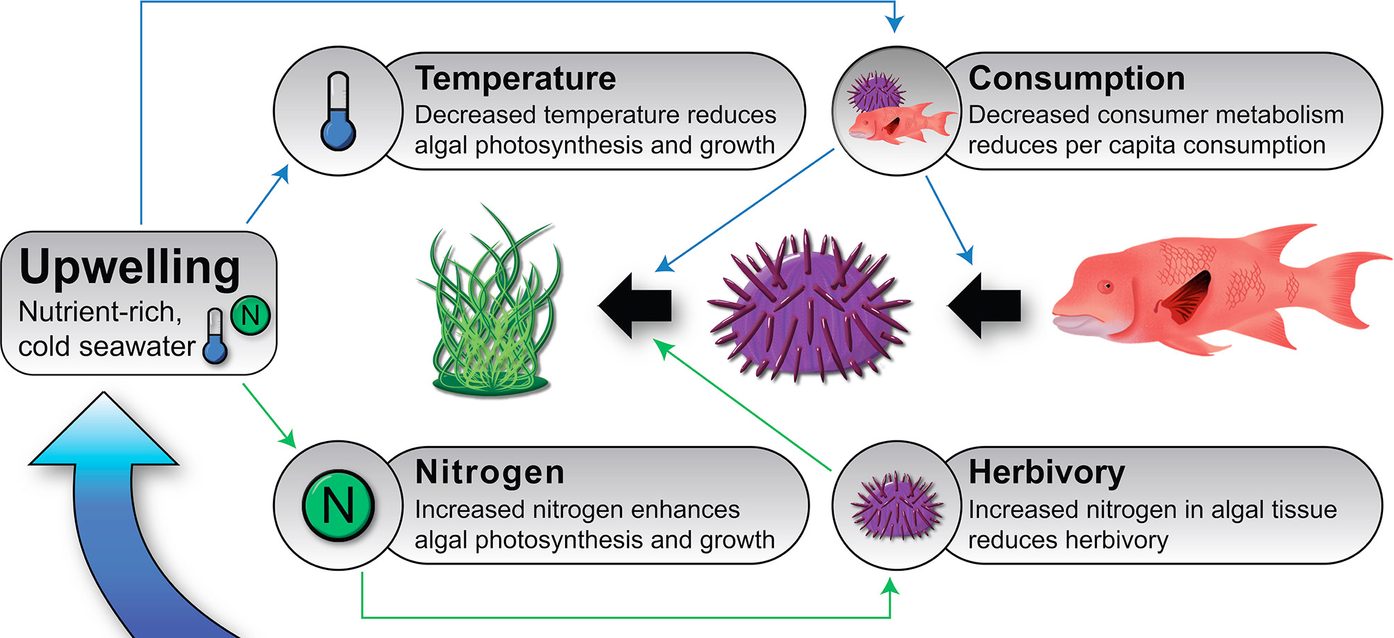
Effects of Herbivory and Nutrients on Algal Growth Rates

Research Context

Researchers have implemented an experiment to evaluate the effects of herbivory and nutrients on algal growth rates. On randomized locations across a reef, they’ve exposed 1x1 m areas to one of 5 treatments:

Full cage
Additional nutrients
Full cage + additional nutrients
An open cage
Control – no manipulation.

The cage represents an herbivore exclusion treatment. The open cage is a control for potential effects of the cage itself.

After 1 month, they measured the growth (in mm) of algae in each treatment, to get the growth rate in mm / month.

Your task is to analyze the data from this experiment and determine the effects of these treatments on algal growth rates.

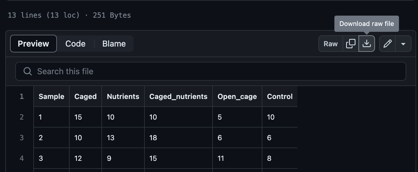
Download the data

Follow the link to Download this data - This will take you to github where you will see option to “Download raw file” on the right side of the window. Shown here:

Steps:

i. Open a new script and make a header: At the top of your R script, include a header with your name, the date, and a brief description of the analysis.

ii. Setting the Working Directory: Set the working directory to where your dataset is located, and where you want to save your scripts and outputs. It is helpful to save these scripts all together so you can come back to them.

iii. Install and load libraries: Load the necessary packages for the exercise. There are a few we have loaded pretty consistently through now, so probably best to load those up.

###########################
# Lab Activity Sept 25 or Week 7
# Author: 
# Date: 
###########################

# set working directory
setwd("set/your/working/directory/here")

# load libraries 
# library(LIBRARY_YOU_NEED1)
# library(LIBRARY_YOU_NEED2)

1. Import the data into RStudio. Melt and rearrange if necessary.

useful commands: read.csv(), pivot_longer()
Once you have the data in your desired format that is able to be analyzed, describe it (complete the sentence, each row in this dataset represents/contains…)

2. Make a summary dataframe of your data.

useful commands: group_by(), summarise()
include the mean, standard deviation, and standard error for each treatment.

3. Using the summary dataframe you just made, plot average algal growth +/- standard error bars.

useful commands: ggplot(), geom_bar(), geom_errorbar()
Based on the graph, do algal growth rates appear to differ among the treatments?

4. Perform an ANOVA on the data.

useful commands: aov()
what are your statistical \(H_0\) and \(H_1\) for the ANOVA test?

5. ANOVA Assumption: Test normality of residuals using the Shapiro-Wilk test.

useful commands: shapiro.test()
What is the null hypothesis of the Shapiro-Wilk test?
Do you accept or reject this hull hypothesis, and what does this mean?

6. ANOVA Assumption: Test homoscedasticity using Bartlett’s test.

useful commands: bartlett.test()
What is the null hypothesis of Bartlett’s test?
Do you accept or reject this hull hypothesis, and what does this mean?

7. Interpret ANOVA results.

print the summary() of the aov, and interpret the output in one sentence.
Do you accept or reject \(H_0\) ? What does this mean about between group and within group variance? Look back at the fundamentals of ANOVA

8. Perform post-hoc Tukey’s HSD test.

useful commands: TukeyHSD(), or HSD.test from library(agricolae) ; remember to load your libraries at the beginning of your script, go back to the top and add agricolae, if you have not already.
In general, what do the results of the Tukey’s HSD test tell you that the overall ANOVA does not?

9. Succinctly (2-4 sentences) discuss the results of the experiment concerning the effects of herbivory and nutrients on algal growth.

For steps 10 and 11, follow the code used in the section immediately before this section. You must modify that code, and fill in the correct terms/variables/columns for this dataset. This is very similar to what you will be doing when you are working on your own data.

10. add a column to your summary dataframe containing significance letters indicating the results of the Tukey HSD test.

11. Add the significance letters to a bar graph to visualize the results.

Brandt, Margarita, Isabel Silva-Romero, David Fernández-Garnica, Esteban Agudo-Adriani, Colleen B. Bove, and John F. Bruno. 2022. “Top-down and Bottom-up Control in the Galápagos Upwelling System.” Frontiers in Marine Science 9 (May). https://doi.org/10.3389/fmars.2022.845635.