In experimental design, we often encounter situations where one factor is nested within another. This hierarchical structure is common in ecological studies, where samples might be collected from different sites within larger regions. Nested ANOVA is a statistical technique that allows us to analyze such hierarchical data structures, providing insights into how variability is distributed across different levels of organization.
Nested Design
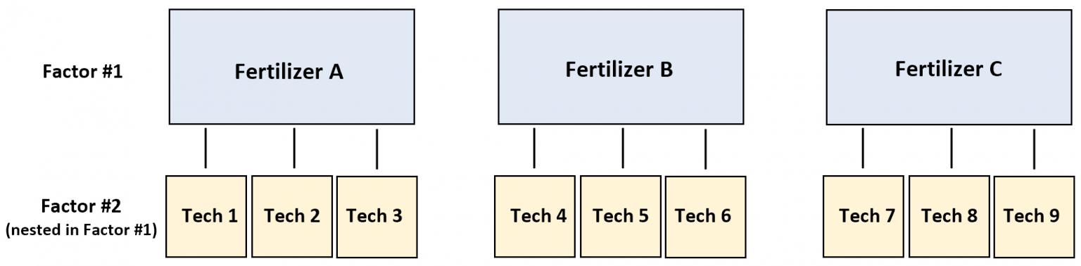
Unlike factorial designs where every level of each factor interacts with every level of the other, nested designs have a hierarchical structure. In the image above, we see technicians nested within fertilizer treatments. This means that each technician works exclusively with one fertilizer type, creating a nested relationship.
The Nested ANOVA Model
The nested ANOVA model can be represented mathematically as:
\(Y_{ijk}\) is the \(k^{th}\) observation within the \(j^{th}\) level of factor B, nested within the \(i^{th}\) level of factor A.
\(\mu\) is the overall mean
\(A_i\) is the effect of the \(i^{th}\) level of factor A
\(B_{j(i)}\) is the effect of the \(j^{th}\) level of factor B, nested within the \(i^{th}\) level of factor A
\(\epsilon_{ijk}\) is the random error
This model allows us to partition the variance between the main factor (A), the nested factor (B), and the residual error, providing a comprehensive view of how different levels contribute to the overall variability in the data.
Implementing Nested ANOVA in R
Let’s work through an example to illustrate how to perform a nested ANOVA in R. We’ll use a simulated dataset representing nitrate levels measured at three different islands, with three reefs sampled within each island.
Data Simulation and Preparation
First, we’ll create a function to simulate our data. Dont worry too much about this for now since its just how we are making up the data
  Island   Reef nitrate_level
1    STT Site 1      5.368437
2    STT Site 2      6.768939
3    STT Site 3      6.661785
4    STT Site 4      4.624343
5    STT Site 5      3.530989
6    STJ Site 6      3.995685
Model Formulation and Analysis
Now, let’s perform the nested ANOVA:
model<-aov(nitrate_level~Island/Reef, data =df)summary(model)
             Df Sum Sq Mean Sq F value   Pr(>F)
Island        2  771.6   385.8  21.531 7.66e-09 ***
Island:Reef  12    9.0     0.7   0.042        1
Residuals   135 2419.1    17.9
---
Signif. codes:  0 '***' 0.001 '**' 0.01 '*' 0.05 '.' 0.1 ' ' 1
In this formula, Island/Reef indicates that Reef is nested within Island. The slash (/) operator in R’s formula notation represents this nesting relationship.
Interpreting the Results
Let’s break down the output of our nested ANOVA:
              Df Sum Sq Mean Sq F value   Pr(>F)
Island        2  864.6   432.3  23.781 1.42e-09 ***
Island:Reef  12   14.4     1.2   0.066        1
Residuals   135 2454.3    18.2
---
Signif. codes:  0 '***' 0.001 '**' 0.01 '*' 0.05 '.' 0.1 ' ' 1
Degrees of Freedom (Df): We have 2 degrees of freedom for Island (3 islands minus 1) and 12 for Reef nested within Island (5 reefs per island * 3 islands, minus 3 islands).
Sum of Squares (Sum Sq): The Island factor accounts for a large portion of the variability (864.6), while the nested Reef factor contributes minimally (14.4).
Mean Square (Mean Sq): This represents the average variability for each factor. For Island, it’s substantial (432.3), but for Reef within Island, it’s quite small (1.2).
F value: The F value for Island (23.781) is large, indicating that differences between islands explain a significant amount of variance. In contrast, the F value for Reef within Island (0.066) is very small.
Pr(>F): The p-value for the Island effect is highly significant (1.42e-09), indicated by the three asterisks. This suggests strong evidence for differences in nitrate levels between islands. However, the Reef within Island effect has a p-value of 1, indicating no significant differences between reefs within the same island.
In our example, the results show that nitrate levels differ significantly between islands. The large F value and small p-value for the Island factor suggest that the variation in nitrate levels is primarily explained by differences between islands.
Interestingly, the Reef within Island factor shows no significant effect. This implies that while nitrate levels vary greatly from one island to another, they are relatively consistent across different reefs within the same island. This could indicate that island-wide factors (such as overall water quality, currents, or island-specific pollution sources) have a stronger influence on nitrate levels than localized factors at the reef level.
These findings highlight the importance of considering broader geographical scales (islands) when studying nitrate levels in this marine environment, as the smaller scale variations (between reefs) appear to be negligible in comparison. This information could be valuable for environmental management strategies, suggesting that island-wide approaches might be more effective than reef-specific interventions for managing nitrate levels in this ecosystem.
Visualization
Visualizing the data can provide additional insights:
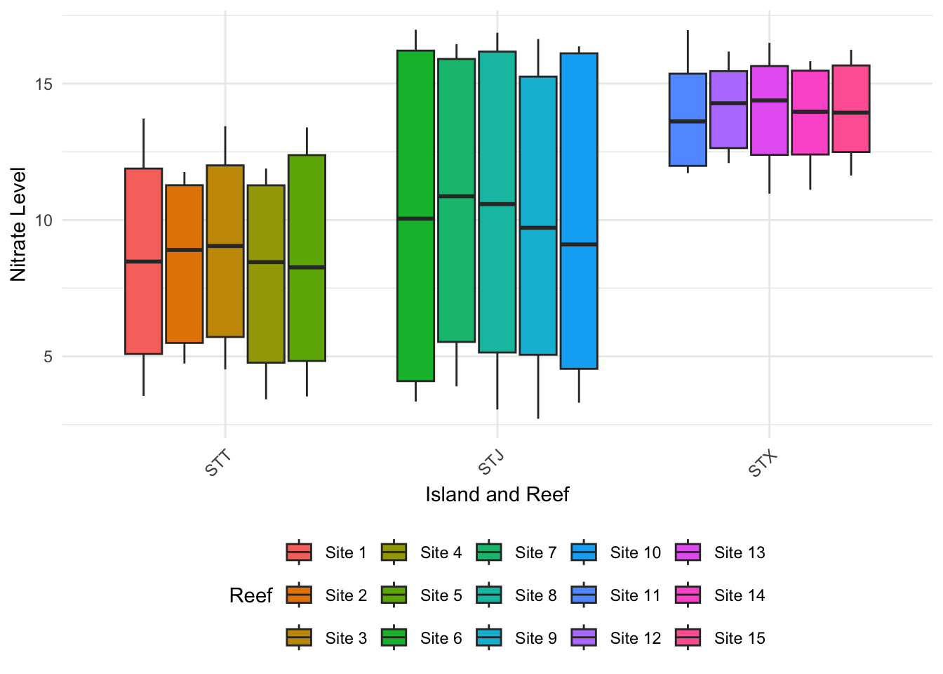
The boxplot provides a visual representation of our nested ANOVA results, effectively illustrating the patterns of nitrate levels across islands and reefs:
Island-level differences: The most striking feature of the plot is the clear separation between nitrate levels across the three islands (STT, STJ, and STX). This visual distinction aligns perfectly with our ANOVA results, which showed a highly significant effect for the Island factor (F = 23.781, p = 1.42e-09). We can see that:
STT (leftmost) has the lowest nitrate levels, generally ranging from about 5 to 10.
STJ (middle) shows intermediate levels, mostly between 10 and 15.
STX (rightmost) exhibits the highest nitrate concentrations, typically between 13 and 17.
Reef-level similarities: Within each island, the boxplots for different reefs (represented by different colors) largely overlap and show similar medians and interquartile ranges. This visual consistency supports our ANOVA finding of a non-significant Reef within Island effect (F = 0.066, p = 1). The similarity of reef-level distributions within each island suggests that nitrate levels are relatively uniform across reefs on the same island.
Variability: The spread of the boxes and whiskers for each reef is comparable, indicating similar variability in nitrate levels across reefs and islands. This consistency in spread supports the use of ANOVA, which assumes homogeneity of variance.
Outliers: A few outliers are visible, particularly for some reefs in STJ and STX. However, these don’t seem to dramatically influence the overall pattern, which is consistent with the strong island-level effect we found in the ANOVA.
Gradual increase: There’s a noticeable trend of increasing nitrate levels as we move from STT to STJ to STX. This gradient further emphasizes the significant island-level differences detected in our analysis.
The visualization thus confirms and elaborates on our statistical findings. It clearly shows that while nitrate levels vary substantially between islands, they remain relatively consistent within each island, regardless of the specific reef. This graphical representation reinforces our conclusion that island-wide factors are the primary drivers of nitrate level variations in this ecosystem, overshadowing any reef-specific effects.
Assumptions and Considerations
When using nested ANOVA, it’s important to consider the following assumptions:
Independence: Observations should be independent within each group.
Normality: Residuals should be normally distributed.
Homogeneity of Variance: Variances should be equal across groups.
Tip
After confirming the absense of a nested effect, such as the Island:Reef interaction in our example, it may be appropriate to pool the data across the nested factor and re-run the ANOVA with only the main factor. This can simplify the analysis and interpretation, especially when the nested factor doesn’t significantly contribute to the variability in the response variable.
Post Hoc Tests
If differences are detected, use post hoc tests (e.g., Tukey’s HSD) to discern which groups significantly differ.
library(emmeans)# getpairs <- emmeans(model, ~ Island/Reef) # if nested effect was significant.getpairs<-emmeans(model, ~Island)tukey<-pairs(getpairs, adjust="tukey")pairs
function (x, ...)
UseMethod("pairs")
<bytecode: 0x136d6c148>
<environment: namespace:graphics>
 contrast  estimate    SE  df t.ratio p.value
 STT - STJ    -1.68 0.847 135  -1.982  0.1206
 STT - STX    -5.43 0.847 135  -6.409  <.0001
 STJ - STX    -3.75 0.847 135  -4.427  0.0001

Results are averaged over the levels of: Reef
P value adjustment: tukey method for comparing a family of 3 estimates
The code snippet getpairs <- emmeans(model, ~ Island) is using the emmeans package in R to compute estimated marginal means (EMMs) for a fitted model with respect to the factor Island. Note that we do not need to consider Reef in the post-hoc test since it was not significant in the nested ANOVA.
After conducting our nested ANOVA, we performed a post-hoc Tukey’s Honest Significant Difference (HSD) test to examine pairwise differences between islands. This test helps us understand which specific islands differ significantly from each other in terms of nitrate levels. Let’s interpret the results:
The estimated difference in nitrate levels between STT and STJ is -2.00 units.
This difference is marginally significant (p = 0.0505), just at the conventional threshold of statistical significance (p < 0.05).
We can interpret this as a trend suggesting that STJ has slightly higher nitrate levels than STT, but the evidence is not strong.
STT vs. STX:
The estimated difference between STT and STX is -5.35 units.
This difference is highly significant (p < 0.0001).
We can confidently say that STX has substantially higher nitrate levels compared to STT.
STJ vs. STX:
The estimated difference between STJ and STX is -3.34 units.
This difference is also highly significant (p = 0.0004).
We can conclude that STX has significantly higher nitrate levels than STJ.
These results paint a clear picture of the nitrate level differences across the three islands:
STT consistently shows the lowest nitrate levels.
STX has the highest nitrate levels, significantly higher than both STT and STJ.
STJ falls in between, with nitrate levels significantly lower than STX but only marginally higher than STT.
This pattern aligns with and further clarifies our earlier ANOVA results, which indicated significant differences between islands. The post-hoc test allows us to pinpoint exactly where these differences lie, revealing a clear gradient of increasing nitrate levels from STT to STJ to STX.
These findings could have important implications for understanding the factors influencing nitrate levels across these islands. The consistent and significant differences suggest that island-specific characteristics (e.g., land use, runoff patterns, or geological features) might play a crucial role in determining nitrate concentrations in the surrounding waters.