  Tukey multiple comparisons of means
    95% family-wise confidence level

Fit: aov(formula = Fish_Biomass ~ MPA_Type, data = data_fish_mpa)

$MPA_Type
                            diff        lwr       upr p adj
notake-limitedtake      12.56745   8.102402  17.03250     0
openaccess-limitedtake -15.57068 -20.035735 -11.10563     0
openaccess-notake -28.13814 -32.603187 -23.67309 0Post Hoc Tests
After conducting an Analysis of Variance (ANOVA) and finding a significant difference among the groups, the next logical question arises: “Which specific groups differ from each other?” This is where post-hoc tests come into play. These tests allow us to make pairwise comparisons between groups while controlling for the increased risk of Type I errors that comes with multiple comparisons.
It’s crucial to remember that post-hoc tests should only be performed following a significant ANOVA result. Conducting them without this prerequisite can inflate the risk of false positives, leading to potentially misleading conclusions.
Tukey’s Honestly Significant Difference (HSD)
One commonly used post-hoc test is Tukey’s Honestly Significant Difference (HSD). This test is particularly useful when you have equal sample sizes and variances among groups, which aligns well with the assumptions of ANOVA. In practice this rule is not always followed.
Purpose: Tukey’s HSD is designed to compare all possible pairs of means while maintaining the family-wise error rate at the desired significance level (usually 0.05).
How it works: The test calculates a critical value that represents the minimum difference between any two group means that is required for statistical significance. If the actual difference between two group means exceeds this critical value, we conclude that those groups are significantly different from each other.
Let’s apply Tukey’s HSD to our fish biomass data:
Interpreting Tukey HSD Output
The Tukey HSD output provides valuable information about the pairwise comparisons between our MPA types. Let’s break down the key components:
Difference (diff): This column shows the difference between the means of two groups. A positive value indicates that the first group has a higher mean than the second, while a negative value suggests the opposite.
95% Confidence Interval (lwr & upr): These columns provide a range within which we can be 95% confident that the true difference between group means lies. If this interval doesn’t include zero, it’s a strong indication that the groups are likely different.
Adjusted p-value (p adj): This value tells us if the observed difference is statistically significant. Typically, we consider differences with p-values less than 0.05 to be significant.
Let’s examine each comparison:
-
No-Take vs. Limited-Take:
- The “No-Take” MPAs have a higher fish biomass by about 12.57 units compared to “Limited-Take” MPAs.
- We’re 95% confident that this difference lies between 8.10 and 17.03.
- The difference is statistically significant (p = 0).
-
Open-Access vs. Limited-Take:
- “Open-Access” MPAs have a lower fish biomass by about 18.89 units compared to “Limited-Take” MPAs.
- The 95% confidence interval for this difference is between -23.35 and -14.42.
- This difference is statistically significant (p = 0).
-
Open-Access vs. No-Take:
- “Open-Access” MPAs have a lower fish biomass by about 31.46 units compared to “No-Take” MPAs.
- We’re 95% confident that this difference is between -35.92 and -26.99.
- The difference is statistically significant (p = 0).
These results provide a nuanced understanding of how fish biomass differs across MPA types. They suggest that No-Take MPAs are the most effective in maintaining high fish biomass, followed by Limited-Take MPAs, with Open-Access areas showing the lowest fish biomass.
This information can be invaluable for conservation planning and policy-making, offering evidence-based insights into the effectiveness of different protection strategies. However, it’s important to consider these statistical findings alongside practical significance and other contextual factors when making decisions.
A more interesting example

That was … boring (made up data often is)
Lets look at another example.
Imagine we weighed 30 turtles that we found at different beaches, and we want to know if there are significant differences in their weights across the beaches. We’ll use a one-way ANOVA to test this hypothesis and then follow up with a Tukey HSD test to identify specific differences between the beaches.
# Set seed for reproducibility
set.seed(123)

# Create a sample dataset of turtle counts per day across different beaches
beach_A <- round(rnorm(30, mean = 17, sd = 2))
beach_B <- round(rnorm(30, mean = 18, sd = 1))
beach_C <- round(rnorm(30, mean = 19, sd = 2))

# Boxplot of the data
boxplot(beach_A, beach_B, beach_C, names = c("A", "B", "C"),
        col = "lightblue", main = "Boxplot of Turtle Weights per Beach",
        ylab = "Turtles weight (kg)")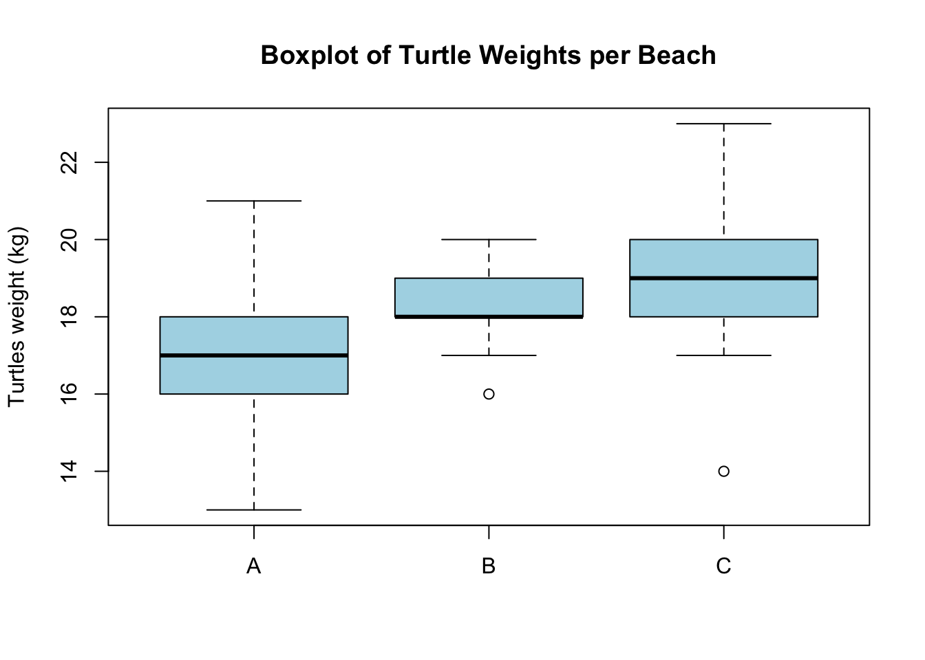
# Combine data into a single dataframe
data <- data.frame(
  turtles = c(beach_A, beach_B, beach_C),
  beach = factor(rep(c("Brewers", "Bald Head", "Tortuga"), each = 30))
)

# Perform one-way ANOVA
anova_result <- aov(turtles ~ beach, data = data)

# Print ANOVA summary
print(summary(anova_result))
Df Sum Sq Mean Sq F value Pr(>F)
beach 2 67.4 33.70 13.41 8.41e-06 ***
Residuals 87 218.7 2.51
---
Signif. codes: 0 '***' 0.001 '**' 0.01 '*' 0.05 '.' 0.1 ' ' 1# Perform Tukey HSD test
tukey_result <- TukeyHSD(anova_result)
# Print the Tukey HSD results
print(tukey_result) Tukey multiple comparisons of means
95% family-wise confidence level
Fit: aov(formula = turtles ~ beach, data = data)
$beach
diff lwr upr p adj
Brewers-Bald Head -1.3 -2.2761414 -0.3238586 0.0058107
Tortuga-Bald Head 0.8 -0.1761414 1.7761414 0.1298910
Tortuga-Brewers 2.1 1.1238586 3.0761414 0.0000052# Visualize the Tukey HSD results
plot(tukey_result)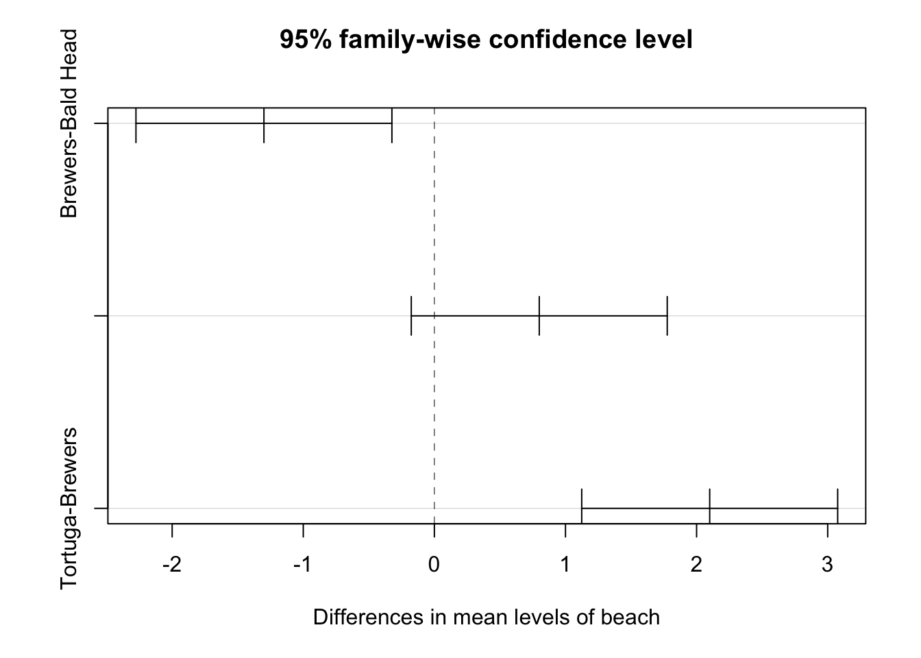
lets interpret!
Beach B vs. Beach A (B-A):
- Difference: 1.3 kg
- 95% Confidence Interval: [0.32386, 2.2761]
- P-value: 0.00581
Interpretation: There is a statistically significant difference in turtle weights between Beach B and Beach A (p < 0.05). On average, turtles on Beach B are 1.3 kg heavier than those on Beach A. We can be 95% confident that the true difference in mean weights is between 0.32 kg and 2.28 kg.
Beach C vs. Beach A (C-A):
- Difference: 2.1 kg
- 95% Confidence Interval: [1.12386, 3.0761]
- P-value: 0.00001
Interpretation: There is a highly statistically significant difference in turtle weights between Beach C and Beach A (p < 0.0001). Turtles on Beach C are, on average, 2.1 kg heavier than those on Beach A. The 95% confidence interval suggests that the true difference in mean weights is between 1.12 kg and 3.08 kg.
Beach C vs. Beach B (C-B):
- Difference: 0.8 kg
- 95% Confidence Interval: [-0.17614, 1.7761]
- P-value: 0.12989
Interpretation: There is no statistically significant difference in turtle weights between Beach C and Beach B (p > 0.05). Although turtles on Beach C are, on average, 0.8 kg heavier than those on Beach B, this difference is not statistically significant. The confidence interval includes zero, which means we cannot rule out the possibility that there’s no real difference in the population means.
Tip
If reporting this in a publication, or thesis, or lab assignment:
An analysis of variance (ANOVA) revealed a significant effect of beach on turtle weights (F(2, 87) = 13.4, p < 0.001).
Tukey’s HSD post-hoc test indicated that turtles from Beach B were significantly heavier than those from Beach A by an average of 1.3 kg (95% CI: 0.32–2.28 kg, p = 0.00581), and turtles from Beach C were significantly heavier than those from Beach A by an average of 2.1 kg (95% CI: 1.12–3.08 kg, p = 0.00001). However, there was no significant difference in turtle weights between Beaches B and C (mean difference: 0.8 kg, 95% CI: -0.18–1.78 kg, p = 0.12989).
In a discussion section, or when thinking about implications, expand on environmental or ecological factors on Beach A which might be leading to lower turtle weights compared to the other two beaches. Further investigation into factors such as food availability, habitat quality, or turtle population demographics on Beach A might be warranted to understand these differences.