Data Transformation in ANOVA

Ensuring your data meets the assumptions of ANOVA makes for reliable results. However, sometimes your data might not naturally meet these assumptions due to outliers, skewness, or other irregularities.

In such cases, transforming your data should be the first thing you try.

Various Data Transformations and Their Implications

Logarithmic Transformation: This is useful when dealing with positively skewed data. It compresses the data, reducing the impact of outliers or large values.

Square Root Transformation: Especially useful for count data, it helps stabilize variances and make the distribution more normal when data is positively skewed.

Square Transformation: Applied when we want to widen the distribution, making it useful for negatively skewed data.

Box-Cox Transformation: A versatile transformation that determines the best power transformation of the data to normalize the distribution.

Choosing a transformation that aligns with your data type and distribution is important to successfully meet the assumptions of ANOVA.

Implementing Data Transformations in R with Examples

In R, data transformation can be smoothly performed with various functions. For instance, if we’re working with a dataset named coral_data…

coral_data <- read.csv("https://raw.githubusercontent.com/laurenkolinger/MES503data/main/week8/coral_data.csv")

head(coral_data)

       Size
1 10.461480
2  6.707424
3 11.627605
4 21.458501
5  6.271983
6  6.272055

---

if we want to apply a logarithmic transformation to the variable Size, we’d do it as follows:

coral_data$Log_Size <- log(coral_data$Size)

head(coral_data)

       Size Log_Size
1 10.461480 2.347700
2  6.707424 1.903215
3 11.627605 2.453382
4 21.458501 3.066121
5  6.271983 1.836093
6  6.272055 1.836104

Note

notice how we are adding another column to the data, not overwriting the original column Size

---

If we want to apply a square root transformation to the Size variable, we can do it as follows:

coral_data$Sqrt_Size <- sqrt(coral_data$Size)

head(coral_data)

       Size Log_Size Sqrt_Size
1 10.461480 2.347700  3.234421
2  6.707424 1.903215  2.589870
3 11.627605 2.453382  3.409927
4 21.458501 3.066121  4.632332
5  6.271983 1.836093  2.504393
6  6.272055 1.836104  2.504407

---

If we want to apply a square transformation to the Size variable, we can do it as follows:

coral_data$Square_Size <- coral_data$Size ^ 2

head(coral_data)

       Size Log_Size Sqrt_Size Square_Size
1 10.461480 2.347700  3.234421   109.44256
2  6.707424 1.903215  2.589870    44.98954
3 11.627605 2.453382  3.409927   135.20119
4 21.458501 3.066121  4.632332   460.46728
5  6.271983 1.836093  2.504393    39.33778
6  6.272055 1.836104  2.504407    39.33868

---

If we want to apply a boxcox transformation to the Size variable, we can do it as follows:

This requires the MASS package, which provides the boxcox() function.

library(MASS)  # Load the MASS package for boxcox()

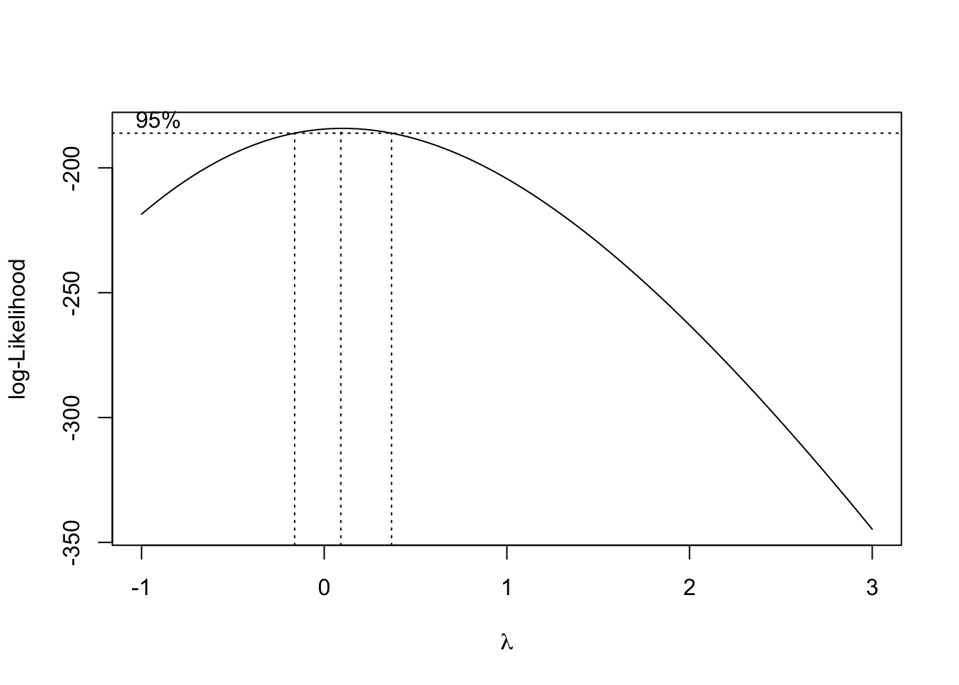
The boxcox() function finds the lambda value that maximizes the log-likelihood for the transformation. We can specify a range of lambda values to search for the optimal transformation. We use the ~ because we are transforming the Size variable without any additional predictors.

boxcox_result <- boxcox(coral_data$Size ~ 1, lambda = seq(-1, 3, 0.1))

Among, other things, this prints out a plot of the log-likelihood values for different lambda values. the best lambda is the one that maximizes the log-likelihood.

Extract the optimal lambda using which.max() on the log-likelihood values (boxcox_result$y).

optimal_lambda <- boxcox_result$x[which.max(boxcox_result$y)]

See if optimal lambda is close to 0 (< 0.0001)

print(optimal_lambda)

[1] 0.09090909

ours is > 0.0001, so we will use the optimal lambda to transform the data.

coral_data$BoxCox_Size <- (coral_data$Size ^ optimal_lambda - 1) / optimal_lambda

head(coral_data)

       Size Log_Size Sqrt_Size Square_Size BoxCox_Size
1 10.461480 2.347700  3.234421   109.44256    2.617048
2  6.707424 1.903215  2.589870    44.98954    2.077783
3 11.627605 2.453382  3.409927   135.20119    2.748504
4 21.458501 3.066121  4.632332   460.46728    3.536076
5  6.271983 1.836093  2.504393    39.33778    1.998225
6  6.272055 1.836104  2.504407    39.33868    1.998238

if the optimal lambda is close to 0, use the log transformation instead (coral_data$Log_Size <- log(coral_data$Size)).

Each transformation modifies the data in a distinct way, making it important to visualize and analyze the transformed data to ensure it meets ANOVA’s assumptions before proceeding with the analysis.

Here are the visualizations of the original and transformed data for a simulated coral_data dataset:

# Loading necessary libraries
library(ggplot2)

# Plotting the original and transformed data
par(mfrow = c(2, 2))  # Setting up a 2x2 plotting grid

# Original Size Data
hist(coral_data$Size, main="Original (Positively Skewed)", xlab="Size", col="skyblue", border="black")

# Log Transformed Data
hist(coral_data$Log_Size, main="Logarithmic Transformation", xlab="Log(Size)", col="skyblue", border="black")

# Square Root Transformed Data
hist(coral_data$Sqrt_Size, main="Square Root Transformation", xlab="Sqrt(Size)", col="skyblue", border="black")

# Box-Cox Transformed Data
hist(coral_data$BoxCox_Size, main="Box-Cox Transformation", xlab="BoxCox(Size)", col="skyblue", border="black")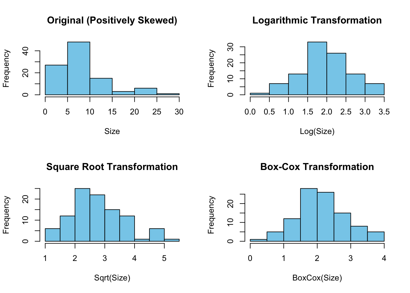

The first plot shows the original data, which is positively skewed. The second plot demonstrates the data after a logarithmic transformation, which compresses the data, reducing the skewness. The third plot presents the data after a square root transformation, also reducing skewness but to a lesser extent compared to logarithmic transformation. The fourth plot displays the data after a Box-Cox transformation, which algorithmically determines the best power transformation to normalize the distribution.