Activity 1: TCRMP Fish
Comparing Fish Abundance and Diversity at TCRMP Sites
Use the template R script copied at the bottom of this page to help complete this activity. For any ALL_CAPS terms, replace or rename them with appropriate terms or more descriptive variable names.
This will be the only time I provide a template, from now on you will start with a blank canvas and some guiding instructions/example commands in the manual
Overview
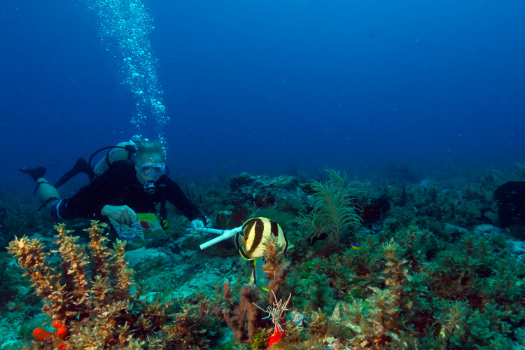
This exercise focuses on the analysis of some fish count data from TCRMP fish surveys. Fish surveys have been historically conducted at 14 sites around St. Croix and 10 sites around St. Thomas and, starting in 2012, are conducted at 32 of the 33 monitoring site. Ten replicate belt transects and three replicate roving dive surveys are conducted at each site. Belt transects are 25 x 4 m and are conducted in 15 minutes per replicate. Roving replicates are also 15 minutes. All fish encountered are recorded except blennies and most gobies.
In this dataset, we are looking at counts of these fish data from sites in 2014 and 2015. You will compare:
fish abundance at Sprat Hole and College Shoal East from surveys conducted in 2014
fish diversity (defined as the number of unique species) at Jacks Bay and Hind Bank East FSA from surveys conducted in 2015.
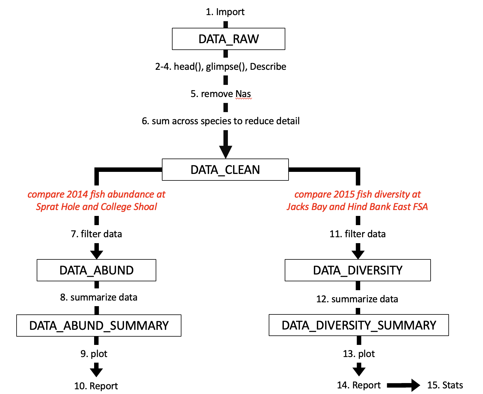
Here is a flow chart showing what your script will be doing.
This week we are doing some exploratory data analysis (EDA). In many ways this approach mirrors data analysis for your thesis data, where you will spend many days/weeks on a single dataset to learn as much about it as you can.
Setup the Script
i. Update the header: At the top of your R script, fill in your name, the date, and a brief description of the analysis.
ii. Set your working directory: Set the working directory to where you want to save your scripts and outputs.
iii. Loading Packages: Load the necessary packages (e.g.,
Tidyverse,dplyr, ggplot2) for the exercise. Make sure you have these installed (install.packages()). Remove or comment outInstall.packages()BEFORE turning in your script.
Import the Data
-
Import the dataset using
read.csv()and give it a descriptive name. We useDATA_RAWin the instructions, but consider being more specific in your naming.
DATA_RAW <- read.csv("https://github.com/laurenkolinger/MES503data/raw/main/week3/s4pt4_fishbiodivCounts_23sites_2014_2015.csv")Explore and Describe the Data
View the First Few Rows of the Dataset using
head(). Pay attention to the column names. There are definitions for those columns in the associated metadata. Click here to download that metadata and save it in your working directory.-
Get a Summary of the Dataset using
summary().What does
summary()tell you? -
Look at the data and metadata, and complete the sentence: “In this data, each row contains ________________”.
Describing the data is an important first step and will be the first step of all activities going forward!
Clean the data
- Remove Missing Values. use this example code to see if any data are NA, and if so, remove them.
-
did
na.omit()work? runwhich(is.na(DATA_RAW), arr.ind = T)to find out.
-
aggregate (condense) counts by summing across species A common practice with this kind of data is to reduce the amount of detail you want to work with in order to answer the question at hand. We have a bunch of cool data on different species, but we dont need this much detail. So we are going to make a second variable
DATA_CLEANto reduce that complexity, by doing some initial “tidying”. Here is example code to get you started, with the answer mostly filled in1. Remember to changeDATA_CLEANto a more descriptive variable name.
Compare fish abundance at Sprat Hole and College Shoal East in 2014
7. Filter Data to include 2014 surveys conducted at Sprat Hole and College Shoal East.
Here is more example code. You will have to change any terms in all caps (e.g., ALL_CAPS) to the correct terms. Starting with a straightforward example:
See here2 for a plain language explanation of this code.
8. Calculate some descriptive statistics for (i.e., summarize) Fish Abundance in 2014, including mean, standard deviation, and SEM.
Think about the goal of this part of the activity. How do you want to group your data, so that you can compare the sites? If done correctly, DATA_ABUND_SUMMARY should only have two rows. Replace GROUPING_VAR with the name of the column corresponding to that grouping variable. Also, what is the measurement that we care about? replace MEASUREDVAR with the name of the column corresponding to that measured variable.
Note: length() calculates the number of observations, useful for statistical calculations like SEM.
9. Visualize Fish Abundance in 2014 with Error Bars. Here is a basic command to start with. Don’t forget to label your axes, and include a descriptive title. You can look up how to do this very easily, for example see the ggplot cheat sheet.
Check that your plot contains all required elements.
# Example Command
ggplot(DATA_ABUND_SUMMARY, aes(x=GROUPING_VAR, y=MEAN_ABUNDANCE)) +
geom_bar(stat="identity") +
geom_errorbar(aes(ymin=MEAN_ABUNDANCE-SEM_ABUNDANCE, ymax=MEAN_ABUNDANCE+SEM_ABUNDANCE), width=.2)10. Interpret differences in fish abundance between sites.
-
Report the calculated means ± SEM as if you were reporting this in a publication, or your thesis:
- Eg. “Surveys in
YEARresulted in an average (± SEM) of ### (± ###) fish at SITE1 and ### (± ###) fish at SITE2.”
- Eg. “Surveys in
Which site had higher fish abundance? Do you think a statistical test would indicate significant differences in their abundances?
Compare fish diversity at Jacks Bay and Hind Bank East FSA in 2015
-
Filter Data by repeating step 7 above, but do not overwrite
DATA_ABUND. Maybe replace_ABUNDwith_DIVERSITYto represent diversity.ImportantNote the different
YEARandSITE1andSITE2that you are looking for in this part! -
Repeat step 8 for diversity
ImportantReplace
GROUPING_VARwith the name of the column corresponding to that grouping variable. Also, what is the measurement that we care about? replaceMEASUREDVARwith the name of the column corresponding to that measured variable. Repeat step 9 to make a plot of fish diversity in 2015.
-
Interpret differences in fish diversity between sites.
Report the calculated means ± SEM.
Which site had higher fish diversity? Do you think a statistical test would indicate significant differences in their diversity?
perform a T test on diversity by site and answer these three questions:
- What are your null and alternative hypotheses?
- Do you reject your null hypothesis?
- Compare this result to what you guessed in 14.
test <-
t.test(
MEASURED_VAR ~ GROUPING_VAR,
data = DATA_DIVERSITY,
var.equal = TRUE
)Template R Script
###########################
# Lab Activity Week 3-4: Summarizing TCRMP Fish Data
# Author: [Your Name]
# Date: [Current Date]
###########################
# Setting Working Directory
setwd("YOUR_WORKING_DIRECTORY")
# Loading Packages
library(dplyr)
library(ggplot2)
# ------------------------------------------------------------------------
# Data Import
# 1. Import the dataset. Change DATA_RAW (and all other names in all caps) to something more descriptive.
DATA_RAW <- read.csv("https://github.com/laurenkolinger/MES503data/raw/main/week3/s4pt4_fishbiodivCounts_23sites_2014_2015.csv")
# ------------------------------------------------------------------------
# Preliminary Data Exploration and Summary
# 2. View the first few rows of the dataset
head(DATA_RAW)
# 3. Get a summary of the dataset.
summary(DATA_RAW)
# [Insert answer to question 3 here]
# 4. Complete the sentence: "In this data, each row contains _____________"
# [Insert answer here]
# ------------------------------------------------------------------------
# Data Cleaning
# 5. Remove Missing Values
# Find out the indices of the NAs
which(is.na(DATA_RAW), arr.ind = T)
# Remove NAs
DATA_RAW <- DATA_RAW |> na.omit()
# [Your answer to question asked in 5 here]
# 6. Aggregate counts by summing across species
DATA_CLEAN <- DATA_RAW |>
  select(site, year, replicate, sppname, counts) |>
  group_by(site, year, replicate) |>
  summarise(
    counts = sum(counts),
    diversity = length(sppname))
# ------------------------------------------------------------------------
# Comparing fish abundance at Sprat Hole and College Shoal East in 2014
# 7. Filter Data for 2014 surveys at Sprat Hole and College Shoal East
DATA_ABUND <- DATA_CLEAN |>
filter(year == YEAR, site %in% c("SITE1", "SITE2"))
# 8. Calculate descriptive statistics for Fish Abundance in 2014
DATA_ABUND_SUMMARY <- DATA_ABUND |>
group_by(GROUPING_VAR) |>
summarize(
MEAN_ABUNDANCE = mean(MEASUREDVAR),
SD_ABUNDANCE = sd(MEASUREDVAR),
SEM_ABUNDANCE = sd(MEASUREDVAR) / sqrt(length(MEASUREDVAR))
)
# 9. Visualize Fish Abundance in 2014 with Error Bars
ggplot(DATA_ABUND_SUMMARY, aes(x=GROUPING_VAR, y=MEAN_ABUNDANCE)) +
geom_bar(stat="identity") +
geom_errorbar(aes(ymin=MEAN_ABUNDANCE-SEM_ABUNDANCE, ymax=MEAN_ABUNDANCE+SEM_ABUNDANCE), width=.2) +
labs(x = "Site", y = "Mean Abundance", title = "Fish Abundance in 2014 at Sprat Hole and College Shoal East")
# 10. Interpret differences in fish abundance between sites
# [Insert answer here]
# ------------------------------------------------------------------------
# Comparing fish diversity at Jacks Bay and Hind Bank East FSA in 2015
# 11. Filter Data for 2015 surveys at Jacks Bay and Hind Bank East FSA
# [Insert code here]
# 12. Calculate descriptive statistics for Fish Diversity in 2015
# [Insert code here]
# 13. Visualize Fish Diversity in 2015 with Error Bars
# [Insert code here]
# 14. Interpret differences in fish diversity between sites
# [Insert answer here]
# 15. Perform a T test on diversity by site
test <-
t.test(
MEASURED_VAR ~ GROUPING_VAR,
data = DATA_DIVERSITY,
na.rm = TRUE, # remove nas? this is redundant here (since you removed nas previously) but helpful for future applications.
var.equal = TRUE
)
# [Insert answer here]
# [Insert answer here]
# [Insert answer here]
# [Insert answer here]-
-
Note:
this makes a new variable, called
diversity, which counts the numbers of species per replicate. This which will assist in part 2 of the activity.This removes columns (
program,month,replicatetype,trophicgroup)by not including them inselect(). Even though this is not an essential step, a cleaner data frame can help you better understand your analysis and focus on the questions at hand.
-
-
This piped command performs a specific data filtering operation using the
dplyrpackage in R. Here’s what it does in plain language:DATA_CLEAN: This is the dataset you’re starting with, presumably after you’ve cleaned it to remove missing values or other unwanted data.|>: This is the “pipe” operator. It takes the output from the command on its left (in this case,DATA_RAW) and “pipes” it into the command on its right (in this case,filter()). Essentially, it’s a way to string multiple commands together in a readable and organized manner.filter(): This function is used to filter rows of a dataset based on certain conditions.year == YEAR: This condition says to keep only the rows where theyearcolumn is equal toYEAR(replace this with the numbered year you want). Numeric data types do not need to be enclosed in quotes. The==is an equality operator, which checks if the value on its left is the same as the value on its right.site %in% c(SITE1, SITE2): This condition says to keep only the rows where thesiteis eitherSITE1orSITE2.The%in%operator checks if a value is part of a set of values (in this case, the set isc("SITE1", "SITE2"). You must replaceSITE1andSITE2with the sites you want to keep (remember perfect syntax/spelling/spaces because computers are dumb). Here, “SITE1” and “SITE2” are string values and thus need to be in quotes.filter(year == YEAR, site %in% c(SITE1, SITE2)): Both conditions are placed within thefilter()function, meaning that the function will keep rows that satisfy both conditions.