model <- lm(plankton_biomass ~ SST, data = plankton_temp_data)Interpreting lm() Outputs
Introduction:
Once a linear regression model has been fit to data, interpreting its output is crucial. The output provides key insights about the relationships between variables, the significance of those relationships, and the overall fit of the model. Here, we’ll discuss how to understand the coefficients, significance values, and the importance of adjusted \(R^2\).
first we need to run the model
here is the full output of the model
summary(model)
Call:
lm(formula = plankton_biomass ~ SST, data = plankton_temp_data)

Residuals:
    Min      1Q  Median      3Q     Max
-60.147 -19.119  -0.594  20.004  52.236

Coefficients:
            Estimate Std. Error t value Pr(>|t|)
(Intercept) 305.2741    14.9359   20.44   <2e-16 ***
SST         -10.2230     0.7161  -14.28   <2e-16 ***
---
Signif. codes:  0 '***' 0.001 '**' 0.01 '*' 0.05 '.' 0.1 ' ' 1

Residual standard error: 27.13 on 39 degrees of freedom
Multiple R-squared:  0.8394,    Adjusted R-squared:  0.8352
F-statistic: 203.8 on 1 and 39 DF,  p-value: < 2.2e-16
summary_model <- summary(model)lets break it down piece by piece:
1. Call
summary_model$calllm(formula = plankton_biomass ~ SST, data = plankton_temp_data)lm: This stands for “linear model.” It indicates that you’ve used thelmfunction, which is R’s standard function for fitting linear regression models.-
formula = plankton_biomass ~ SST:The formula specifies the relationship being modeled.
The variable to the left of the
~(in this case,plankton_biomass) is the dependent variable (or the response variable). This is what you’re trying to predict or explain.The variable to the right of the
~(here,SST) is the independent variable (or predictor or explanatory variable). You’re using this variable to predict or explain variations in the dependent variable.The
~symbol can be read as “is modeled as” or “is explained by”. So, in this context, the formula is saying: “plankton_biomass is modeled as a function of SST.”
-
data = plankton_temp_data:This specifies the dataset used to fit the model.
All variables referenced in the formula (
plankton_biomassandSST) are columns within this dataset.
In essence, the model call is telling you: “I’ve fit a linear model where I’m trying to predict or explain plankton_biomass using SST as a predictor, and the data for this analysis comes from the plankton_temp_data dataset.”
2. Residuals
         0%         25%         50%         75%        100%
-60.1471330 -19.1192920  -0.5943754  20.0035593  52.2357745
The summary of residuals provides a sense of how well the model fits the data:
If the residuals are symmetrically distributed around zero, it suggests a good model fit. In this case, the median is close to zero, indicating a reasonably symmetrical distribution.
The range between the minimum and maximum residuals gives an idea of the spread of the residuals. Large residuals may indicate potential outliers or areas where the model isn’t capturing the underlying trend well.
Quartiles help in understanding the distribution of errors. If, for instance, the 1Q and 3Q values are close to zero, it indicates that the majority of the predictions are close to the actual values.
3. Coefficients, their estimates, errors, and statistics
summary_model$coefficients Estimate Std. Error t value Pr(>|t|)
(Intercept) 305.2741 14.9358959 20.43896 1.923230e-22
SST -10.2230 0.7161214 -14.27551 4.501853e-17Intercept:
Estimate (Coefficient): 305.2741
This is the expected value of the dependent variable when all independent variables in the model (in this case, just SST) are 0. Practically, if SST were 0°C, the expected value of the dependent variable (let’s say plankton biomass) would be 305.2741 units (e.g., mg/m^3).
Std. Error: 14.9358959
The standard error provides a measure of the variability or uncertainty around the estimate of the intercept. It tells us how much we’d expect the estimated intercept to vary if we took multiple samples from the population and built a regression model for each sample.
t value: 20.43896
The t-statistic is the ratio of the departure of the estimated value of a parameter from its hypothesized value to its standard error. For the intercept, it tests the null hypothesis that the true intercept is zero. A t-value this large suggests that the intercept is significantly different from zero.
Pr(>|t|): 1.923230e-22 (p-value)
This is an extremely small p-value, indicating very strong evidence against the null hypothesis that the true intercept is zero. Practically, it means the intercept of 305.2741 is statistically significant.
SST (Slope):
Estimate (Coefficient): -10.2230
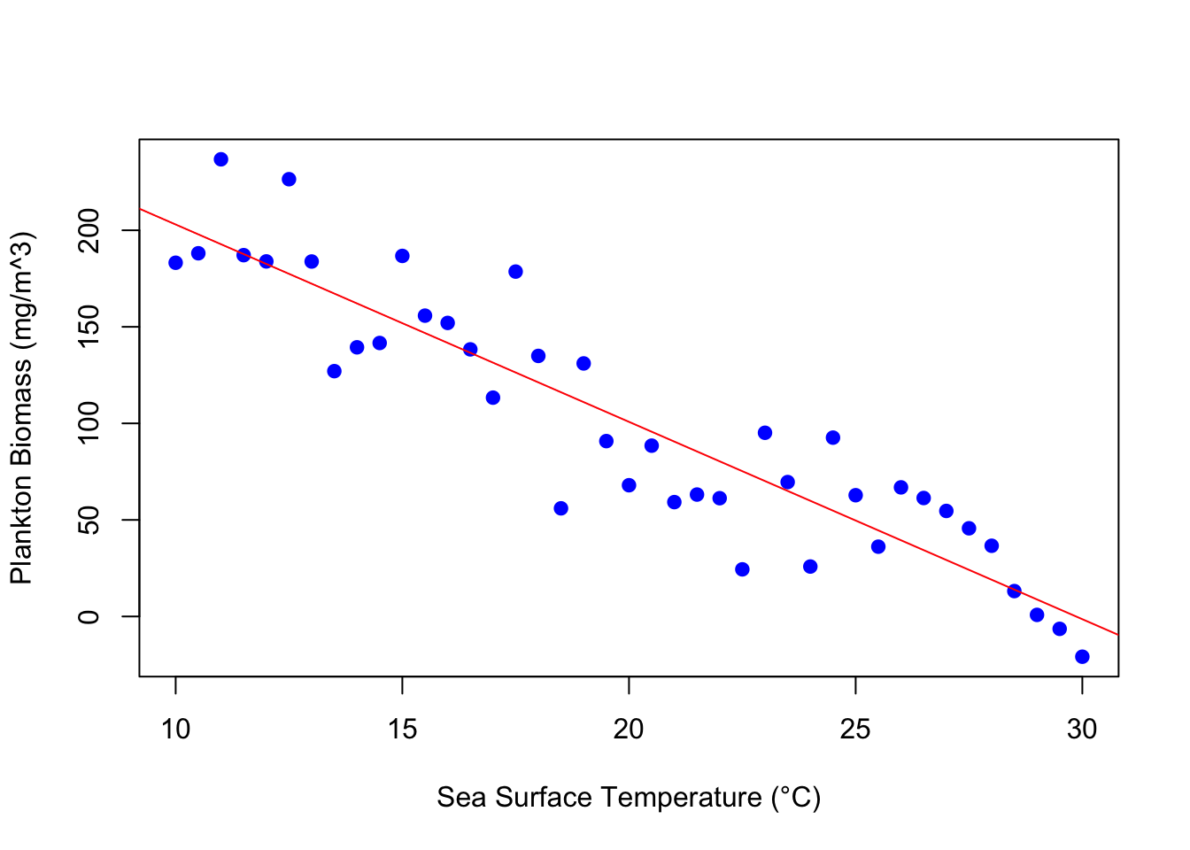
Interpretation: This coefficient represents the change in the dependent variable for a one-unit change in SST, holding other factors constant. Specifically, for every 1°C increase in SST, the plankton biomass decreases by approximately 10.2230 units (e.g., mg/m^3).
Std. Error: 0.7161214
Interpretation: The standard error gives an idea of the variability or uncertainty around the slope estimate. It shows how much we’d expect this estimate to vary across different samples from the population.
t value: -14.27551
Interpretation: This t-statistic tests the null hypothesis that the true coefficient for SST is zero (i.e., SST has no effect). The large magnitude of the t-value and its negative sign aligns with the negative coefficient, indicating a strong and negative relationship between SST and the dependent variable.
Pr(>|t|): 4.501853e-17 (p-value)
Interpretation: This extremely small p-value provides strong evidence against the null hypothesis that SST has no effect on the dependent variable. It confirms that the relationship we observed (the slope) is statistically significant and not due to random chance.
In summary:
The intercept gives us the expected value of the dependent variable when the independent variables are zero.
The slope (for SST) tells us how much the dependent variable changes for a one-unit change in SST.
The standard error gives an indication of the reliability of these coefficients.
The t-statistic tests the hypothesis that the actual coefficient is zero (no effect). A large t-statistic means the coefficient is statistically significant.
The p-value provides the probability of observing the t-statistic if the true coefficient was zero. A small p-value (typically < 0.05) means we can reject this null hypothesis and conclude the coefficient is significant
4. Residual Standard Error
[1] "Residual standard error: 27.13 on 39 degrees of freedom"Residual standard error: 27.13
The residual standard error (RSE) is an estimate of the standard deviation of the residuals—the differences between observed and predicted values. In this context, an RSE of 27.13 means that, on average, the observed values deviate from the values predicted by the model by approximately 27.13 units.
Practically, this gives you a sense of how close (or far) the data points are from the regression line. A smaller RSE indicates that the data points are closer to the fitted line, suggesting a better fit. Conversely, a larger RSE indicates more spread in the residuals, suggesting that the model might not be capturing some of the variability in the data.
39 degrees of freedom
- Degrees of freedom (df) is a concept that represents the number of independent values that can vary in the calculation of a statistic. When fitting a linear regression model, the degrees of freedom is calculated as \(df=n−p−1\), where \(n\) is the number of observations and \(p\) is the number of predictors (excluding the intercept).
- The degrees of freedom is crucial when conducting hypothesis tests or constructing confidence intervals. It affects the critical values of various test statistics. In the context of linear regression, it’s primarily used to determine the significance of predictors by comparing the t-statistic of a coefficient to a t-distribution with a specified number of degrees of freedom.
5. R squared (multiple and adjusted)
[1] "Multiple R-squared: 0.8394, Adjusted R-squared: 0.8352"Both the \(R^2\) and Adjusted \(R^2\) values are measures of model fit.
Multiple \(R^2\): 0.8394
The Multiple \(R^2\) (often just referred to as \(R^2\) or the coefficient of determination) is a measure of the proportion of the variance in the dependent variable that’s predicted by the independent variables.
In this context, an \(R^2\) of 0.8394 means that the model explains approximately 83.94% of the variability in the dependent variable.
Practically, this is considered a high \(R^2\) value, suggesting that the predictors in the model capture a substantial portion of the variability in the dependent variable. However, a high \(R^2\) does not necessarily mean the model is perfect or that there isn’t room for improvement. It simply quantifies the proportion of variance explained.
Adjusted \(R^2\): 0.8352
While the regular \(R^2\) always increases as you add more predictors to your model (even if they are not particularly meaningful), the Adjusted \(R^2\) compensates for this. It takes into account the number of predictors in the model and adjusts the \(R^2\) accordingly.
Adjusted \(R^2\) can be interpreted as the proportion of variation explained by the model, adjusted for the number of predictors. It’s especially useful when comparing models with different numbers of predictors.
An Adjusted \(R^2\) of 0.8352 means that after adjusting for the number of predictors, the model still explains approximately 83.52% of the variability in the dependent variable.
The fact that the Adjusted \(R^2\) is close to the Multiple \(R^2\) suggests that the predictors in the model are relevant and not just inflating the \(R^2\) value.
6. F-statistic and p-value
[1] "F-statistic: 203.8 on 1 and 39 DF, p-value: < 2.2e-16"F-statistic: 203.8 on 1 and 39 DF
The F-statistic is a test statistic used to determine if there’s a relationship between the dependent variable and the independent variables as a whole. It does this by comparing the fit of the model you’ve specified to a model with no predictors (a null model).
In the context of simple linear regression, where there’s only one predictor, the F-test is essentially testing whether this predictor is significant in predicting the outcome variable or not.
The degrees of freedom associated with the F-statistic are given “on 1 and 39 DF”. The first number (1) represents the number of predictors in the model (excluding the intercept), and the second number (39) represents the residual degrees of freedom (related to the number of observations minus the number of predictors minus one).
An F-statistic of 203.8 is quite large, suggesting that the variability explained by the model is significantly greater than the residual variability (i.e., the variability not explained by the model).
p-value: < 2.2e-16
The p-value associated with the F-statistic tests the null hypothesis that all of the regression coefficients are equal to zero versus at least one of them is not. A very small p-value indicates that the predictors in the model are statistically significant in explaining the variation in the dependent variable compared to a model with no predictors.
In this case, a p-value of less than \(2.2×10^{−16}\) is extremely close to zero. This provides very strong evidence against the null hypothesis, suggesting that the model with the predictor (or predictors) is a better fit than a model without any predictors.
Typically, a p-value below 0.05 is considered evidence to reject the null hypothesis. Here, the p-value is way below this threshold, indicating strong statistical significance.
Consider these outputs in the context of the plotted data Figure 1