install.packages("rmarkdown")Introduction to R Markdown and Quarto
Note: R markdown will continue to be used, and this lesson is valuable to you, but I recommend Quarto. Quarto was announced at the 2022 R conference and is considered “the next generation” of R markdown. To learn more, see this FAQ .
R markdown and Quarto are very similar, so this is still a useful lesson, but you can easily switch over to using quarto once you start working on your own projects/analyses.
Markdown
Markdown is a lightweight markup language with plain text formatting syntax. It’s designed to be easy to write and easy to read, making it a popular choice for writing documentation, notes, and web content.
It’s used extensively throughout the internet, from social media platforms to coding repositories, and even in cutting-edge AI applications.
In fact, you’ve likely encountered Markdown without even realizing it. When you use certain formatting options on Reddit or GitHub, you’re using Markdown. Even the outputs from AI models like ChatGPT often utilize Markdown for structure and formatting. Its simplicity and versatility have made it the go-to choice for content creators, developers, and tech enthusiasts alike.
Check out this tutorial if you want to practice markdown
R Markdown
R Markdown is a document format that enables the integration of R code into a markdown document. It combines the core syntax of markdown (an easy-to-write plain text format) with embedded R chunks, allowing for the creation of dynamic documents that can both tell a story and run R code to produce analyses, visualizations, and more.
Why Use R Markdown?
Reproducibility: R Markdown documents are completely reproducible. When you share an R Markdown file, others can rerun the R code to obtain the same results.
Multiple Output Formats: From a single R Markdown document, you can produce a variety of outputs, including HTML, PDF, and Word documents.
Integration: Combine your narrative with R code. This means the text, R code, and results can all be found in one document, making for a neat, integrated workflow.
Getting Started with R Markdown
-
Installation: If you haven’t already, you’ll need to install the
rmarkdownpackage:
-
Creating a New R Markdown Document:
-
In RStudio, go to
File->New File->R Markdown.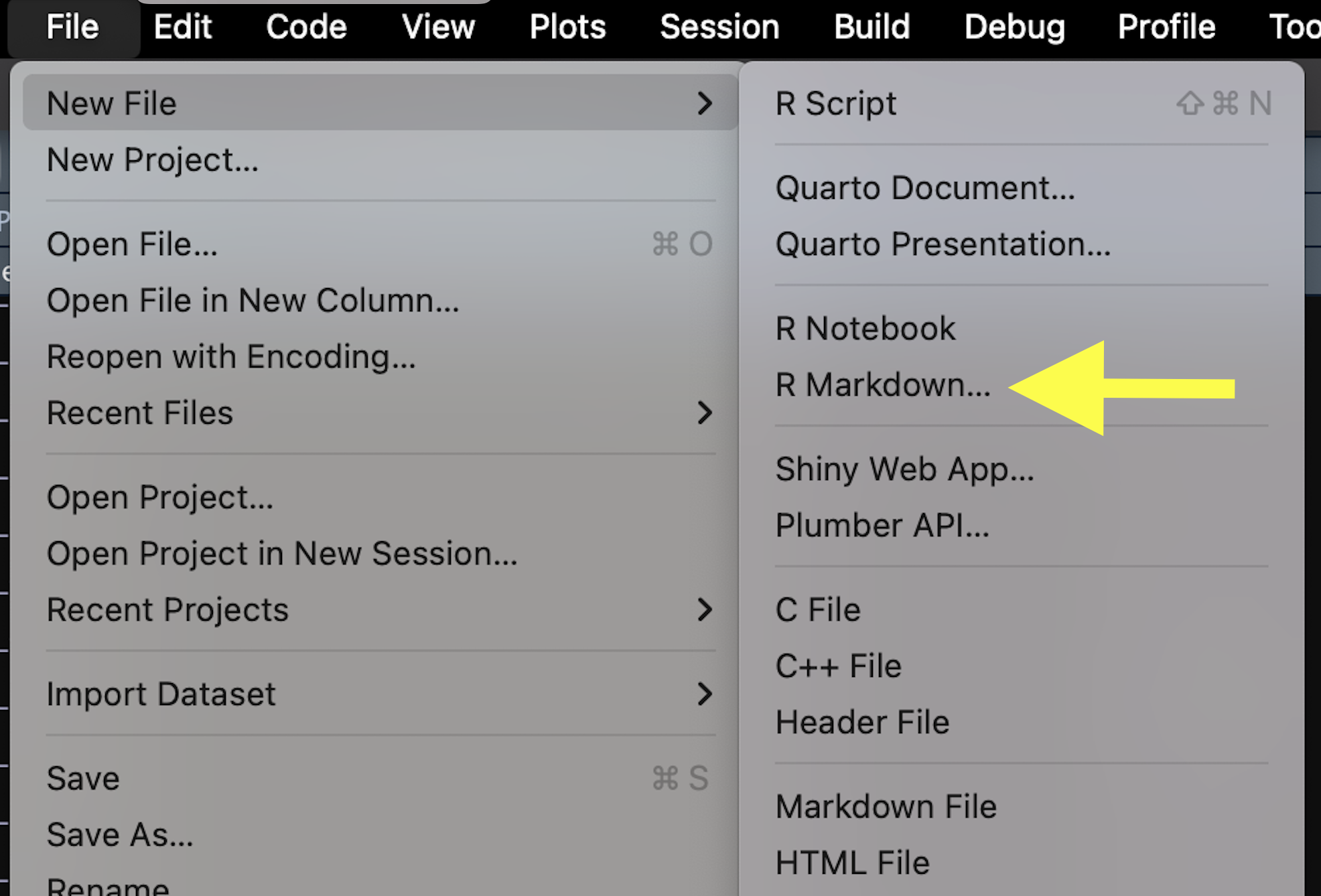
-
You’ll then see a dialog box. For now, keep the default output format as
HTMLand pressOK.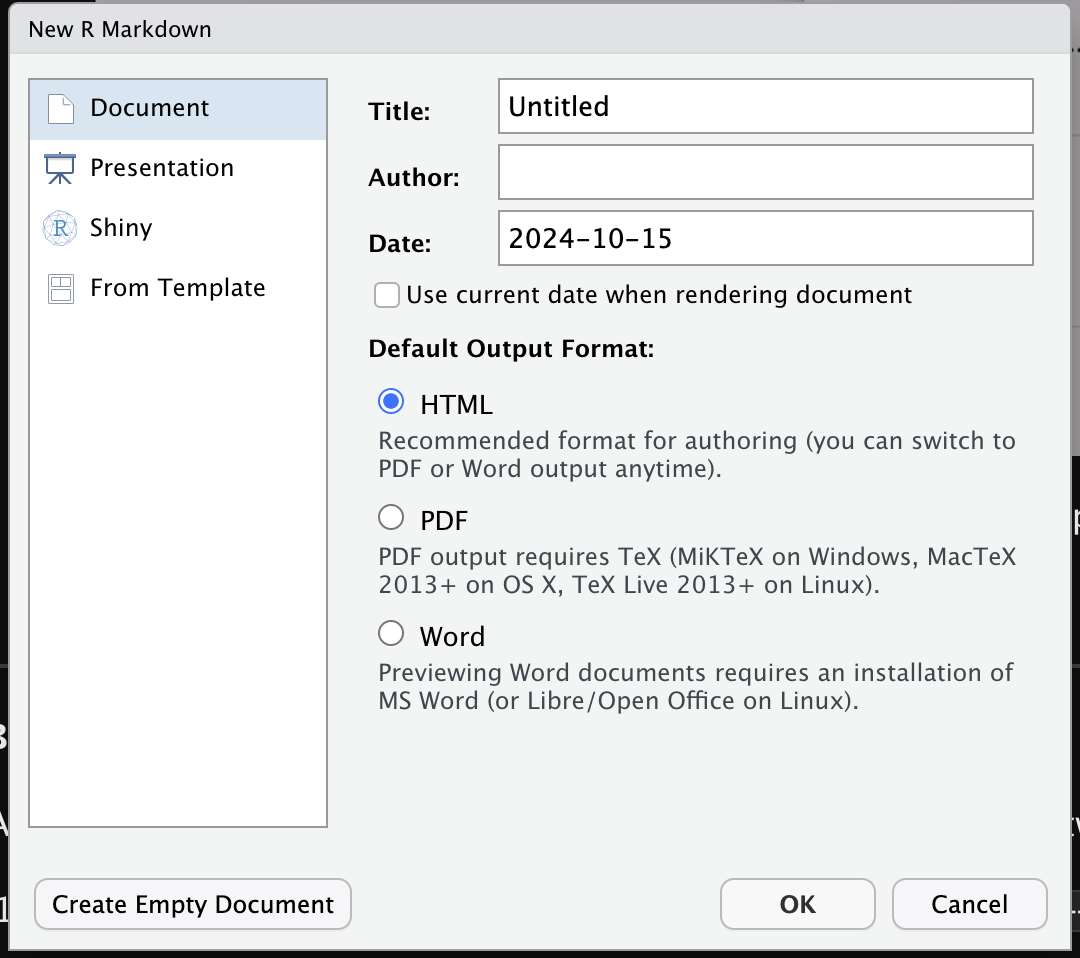
-
this will open up a new R Markdown file in the RStudio script editor
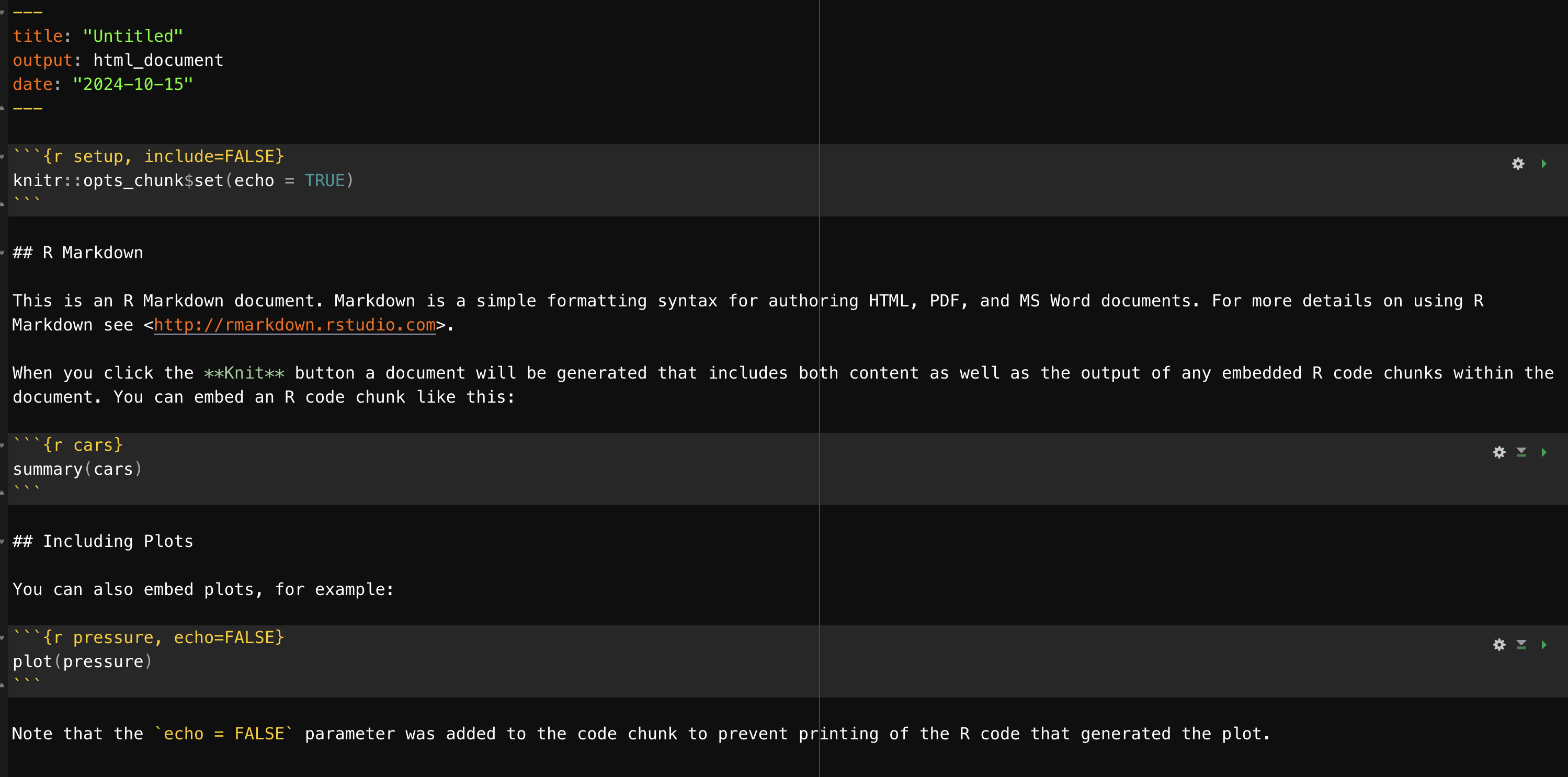
it will have lots of info and examples to start you off
Basic Components of an R Markdown File
An R Markdown file has the extension .Rmd. It’s structured into two main parts:
-
YAML Header: At the top of the document, surrounded by
---, it contains meta-information and settings for the document, such as its title and output format.
---
title: "Your Document Title"
author: "Your Name"
date: "The Date"
output: html_document
---
yaml stands for “YAML Ain’t Markup Language” and is a human-readable data serialization language. It’s used to specify metadata and settings for the document. here, you can set things like the title, author, date, and output format, as well as other options like the theme, font size, and more.
fun fact
This lab manual has its own yaml file that I update each week to add content to.
- Body: This contains the content of the document, with a mix of markdown text and R code chunks.
Formatting in R Markdown
Headers: Use
#for a main header,##for a sub-header,###for a sub-sub-header, and so on.Bold and Italics: Surround text with
**for bold and*for italics.Lists: Use
-or*for bullet points.Links: Format links like this:
[Link Text](URL).
R Code Chunks
R code is inserted into R Markdown documents using code chunks, which are surrounded by three backticks and the letter r in curly braces, like this:
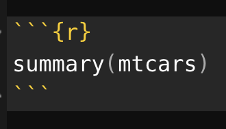
this produces the following visual appearance when rendered, or knitted
summary(mtcars) mpg cyl disp hp
Min. :10.40 Min. :4.000 Min. : 71.1 Min. : 52.0
1st Qu.:15.43 1st Qu.:4.000 1st Qu.:120.8 1st Qu.: 96.5
Median :19.20 Median :6.000 Median :196.3 Median :123.0
Mean :20.09 Mean :6.188 Mean :230.7 Mean :146.7
3rd Qu.:22.80 3rd Qu.:8.000 3rd Qu.:326.0 3rd Qu.:180.0
Max. :33.90 Max. :8.000 Max. :472.0 Max. :335.0
drat wt qsec vs
Min. :2.760 Min. :1.513 Min. :14.50 Min. :0.0000
1st Qu.:3.080 1st Qu.:2.581 1st Qu.:16.89 1st Qu.:0.0000
Median :3.695 Median :3.325 Median :17.71 Median :0.0000
Mean :3.597 Mean :3.217 Mean :17.85 Mean :0.4375
3rd Qu.:3.920 3rd Qu.:3.610 3rd Qu.:18.90 3rd Qu.:1.0000
Max. :4.930 Max. :5.424 Max. :22.90 Max. :1.0000
am gear carb
Min. :0.0000 Min. :3.000 Min. :1.000
1st Qu.:0.0000 1st Qu.:3.000 1st Qu.:2.000
Median :0.0000 Median :4.000 Median :2.000
Mean :0.4062 Mean :3.688 Mean :2.812
3rd Qu.:1.0000 3rd Qu.:4.000 3rd Qu.:4.000
Max. :1.0000 Max. :5.000 Max. :8.000 Compiling the Document
Once you’ve written your R Markdown file, press the “Knit” button in the toolbar at the top of the script editor. This will compile your R Markdown into your chosen output format.
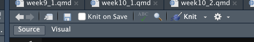
In quarto, I use the “render” button instead, to render the lab manual.
Further Reading
For more detailed tutorials and references on R Markdown, the official R Markdownwebsite is a fantastic resource.

