Non-Parametric Tests When Assumptions are not Met

Sometimes our data doesn’t want to play by the ANOVA rules, even after attempting transformations. In such cases, non-parametric tests become the next step, allowing us to analyze data without being tightly bound to stringent assumptions like normality. These tests employ different mathematical approaches to assess group differences, making them particularly useful when dealing with ordinal or non-normally distributed data.

Common Non-Parametric Alternatives to ANOVA

Kruskal-Wallis Test: This test is a non-parametric alternative to one-way ANOVA. It compares the medians of three or more independent groups to determine if there are statistically significant differences between them. The test assumes that the observations are independent, the groups are mutually independent, and the data is at least ordinal. It does not assume normality or equal variances. However, the test does assume that the distributions of the groups have the same shape and spread, even if they are shifted up or down.

Wilcoxon’s Signed-Ranks Test: This test is a non-parametric alternative to the paired samples t-test. It compares two related samples to assess whether their population mean ranks differ. The test assumes that the differences between pairs are from a continuous and symmetric distribution. It does not assume normality. The test works by calculating the differences between each set of pairs, ranking the absolute values of these differences, and then summing the ranks for the positive and negative differences separately.

Mann-Whitney U Test: This test is a non-parametric alternative to the independent samples t-test. It compares two independent groups to determine if there is a significant difference between them. The test assumes that the observations are independent, the data is at least ordinal, and under the null hypothesis, the distributions of both groups are equal. It does not assume normality or equal variances. The test works by ranking all the observations from both groups, and then summing the ranks for each group. If the sums are very different, the test concludes that the groups are different.

Friedman’s Test: This test is a non-parametric alternative to the one-way repeated measures ANOVA. It is used to detect differences in treatments across multiple test attempts. The test assumes that the data is at least ordinal, the groups are mutually independent, and the responses are measured on the same subjects (or matched subjects) across the different treatments. It does not assume normality or sphericity (equality of variances of the differences between treatments). The test works by ranking each block of subjects separately, then considering the values of ranks by treatments.

Each test has its own specifics regarding the kinds of data and experimental designs it’s suited for, hence choosing the right one is crucial to accurately interpreting your findings.

Implementing Non-parametric Tests in R

Here are simplified R snippets to implement these tests:

# Kruskal-Wallis Test
kruskal.test(ResponseVar ~ GroupVar, data = your_data)

# Wilcoxon's Signed-Ranks Test
wilcox.test(your_data$Var1, your_data$Var2, paired = TRUE)

# Mann-Whitney U Test
wilcox.test(ResponseVar ~ GroupVar, data = your_data, exact = FALSE)

# Friedman's Test
friedman.test(ResponseVar ~ GroupVar | SubjectVar, data = your_data)

Real-World Examples

Kruskal-Wallis Test

Consider an experiment where we tested the effect of three different light conditions on coral growth. The response variable (growth) is not normally distributed among the groups.

# R code for Kruskal-Wallis Test
set.seed(42)  # for reproducibility
coral_growth <- data.frame(
  Growth = c(runif(30, 5, 15), runif(30, 10, 20), runif(30, 15, 25)),
  LightCondition = rep(c("Low", "Medium", "High"), each=30)
)

# Visualizing the data
boxplot(Growth ~ LightCondition, data = coral_growth, main="Coral Growth under Different Light Conditions", ylab="Growth", xlab="Light Condition")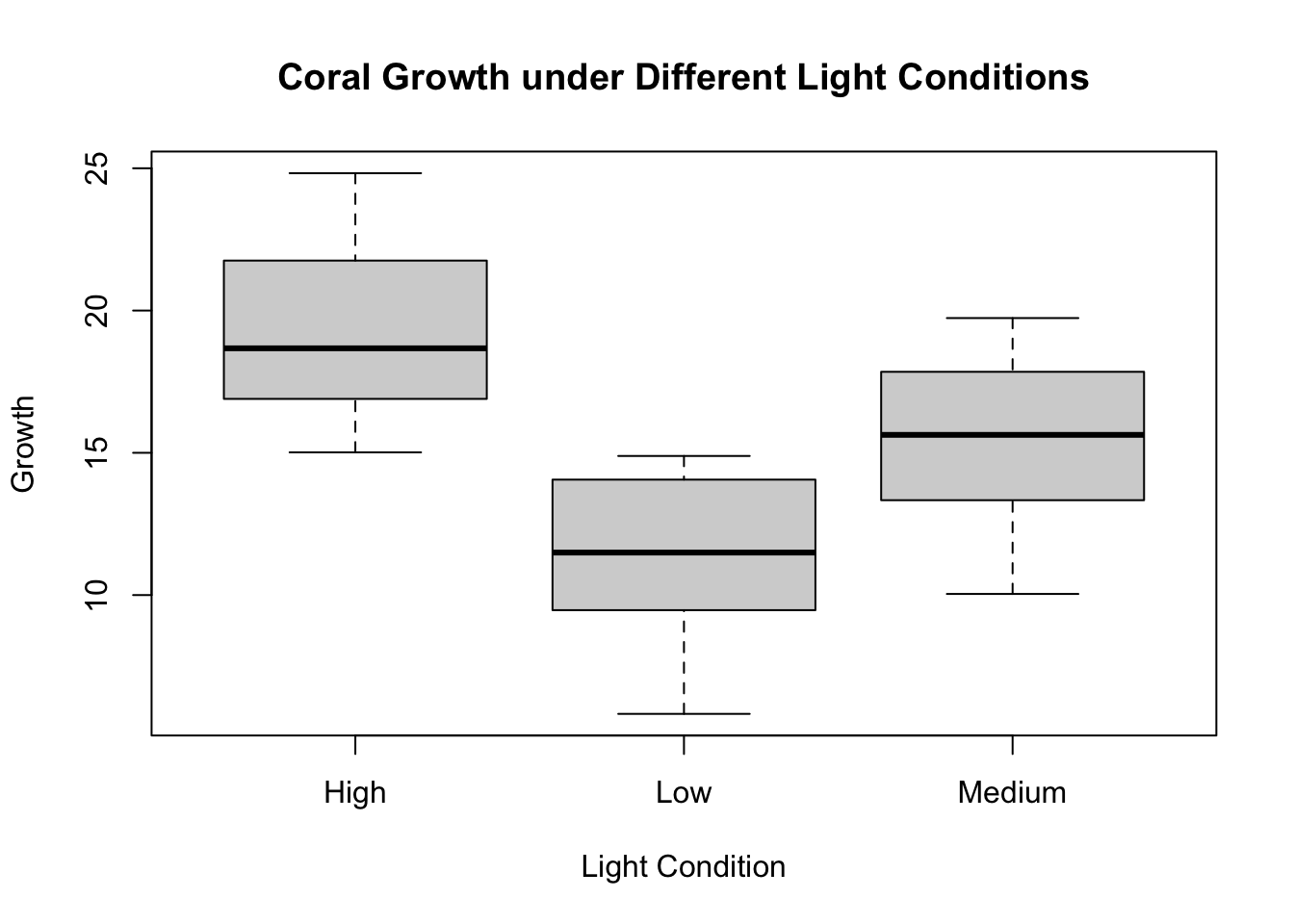

# Performing Kruskal-Wallis Test
kruskal_test_result <- kruskal.test(Growth ~ LightCondition, data = coral_growth)
print(kruskal_test_result)

    Kruskal-Wallis rank sum test

data:  Growth by LightCondition
Kruskal-Wallis chi-squared = 51.916, df = 2, p-value = 5.329e-12

Wilcoxon’s Signed-Ranks Test

Imagine we’re investigating the impact of a treatment on the growth of a coral species, measured before and after the treatment, and our data is not normally distributed.

# R code for Wilcoxon's Signed-Ranks Test
set.seed(42)
coral_treatment <- data.frame(
  GrowthBefore = runif(30, 5, 15),
  GrowthAfter = runif(30, 10, 20)
)

# Visualizing the data
boxplot(coral_treatment, main="Coral Growth Before and After Treatment", ylab="Growth")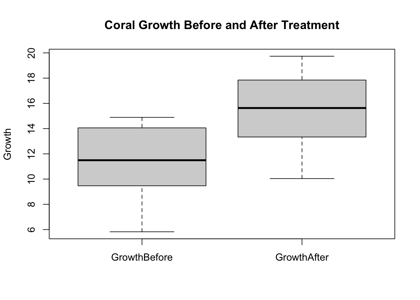

# Performing Wilcoxon's Signed-Ranks Test
wilcoxon_test_result <- wilcox.test(coral_treatment$GrowthBefore, coral_treatment$GrowthAfter, paired = TRUE)
print(wilcoxon_test_result)

    Wilcoxon signed rank exact test

data:  coral_treatment$GrowthBefore and coral_treatment$GrowthAfter
V = 32, p-value = 5.145e-06
alternative hypothesis: true location shift is not equal to 0

Mann-Whitney U Test

Suppose we are comparing the growth rates of two species of coral, without assuming normality in their growth distributions.

# R code for Mann-Whitney U Test
set.seed(42)
coral_species <- data.frame(
  Growth = c(runif(30, 5, 15), runif(30, 10, 20)),
  Species = rep(c("Species_A", "Species_B"), each=30)
)

# Visualizing the data
boxplot(Growth ~ Species, data = coral_species, main="Growth of Two Coral Species", ylab="Growth", xlab="Species")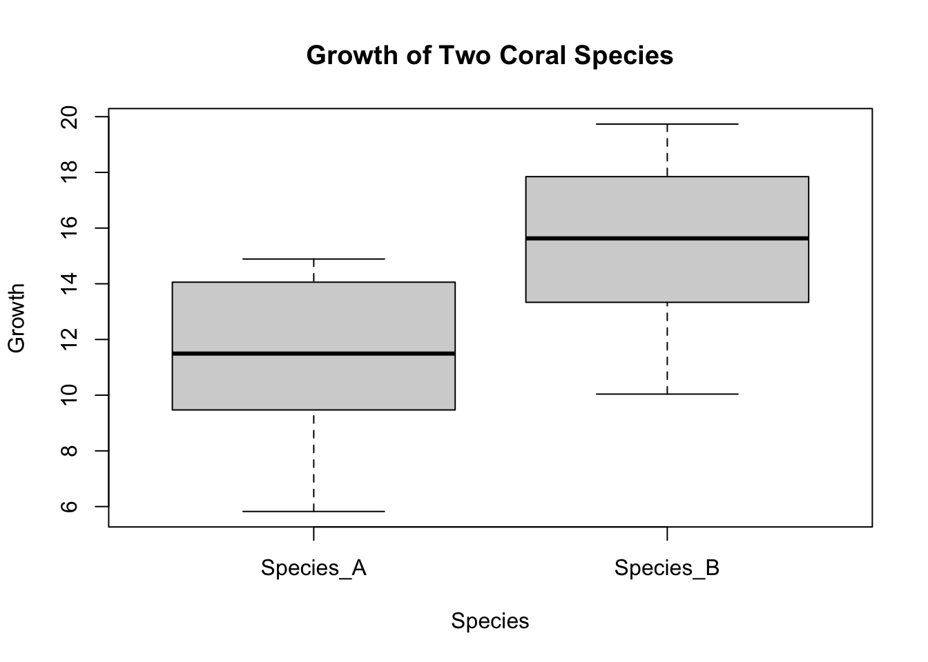

# Performing Mann-Whitney U Test
mann_whitney_test_result <- wilcox.test(Growth ~ Species, data = coral_species, exact = FALSE)
print(mann_whitney_test_result)

    Wilcoxon rank sum test with continuity correction

data:  Growth by Species
W = 167, p-value = 2.959e-05
alternative hypothesis: true location shift is not equal to 0

Friedman’s Test

Imagine we have coral growth data under three different temperature conditions, measured on the same coral colonies, and we want to compare the growth rates.

# R code for Friedman's Test
set.seed(42)
coral_temp <- data.frame(
  Growth = c(runif(30, 5, 15), runif(30, 10, 20), runif(30, 15, 25)),
  Temperature = rep(c("Low", "Medium", "High"), each=30),
  Colony = rep(1:30, times=3)
)

coral_temp$Temperature <- factor(coral_temp$Temperature, levels = c("Low", "Medium", "High"))

# Visualizing the data, using an interaction plot
interaction.plot(coral_temp$Temperature, coral_temp$Colony, coral_temp$Growth, main="Coral Growth under Different Temperatures", ylab="Growth", xlab="Temperature", legend=FALSE)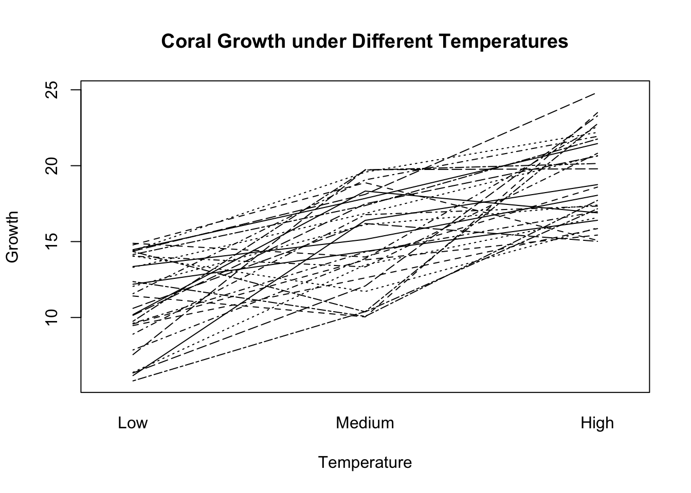

# Performing Friedman's Test
friedman_test_result <- friedman.test(Growth ~ Temperature | Colony, data = coral_temp)
print(friedman_test_result)

    Friedman rank sum test

data:  Growth and Temperature and Colony
Friedman chi-squared = 43.8, df = 2, p-value = 3.083e-10