shapiro.test(data$column_name)T-Tests
Overview
A t-test is a fundamental statistical procedure used to determine if there is a significant difference between the means of two groups. This test is based on the t-distribution, which resembles the normal distribution but accounts for the variability introduced by smaller sample sizes. T-tests are crucial tools across scientific disciplines, providing a robust method to make inferences about populations based on sample data.
T-tests offer an effective way to compare data between two conditions, locations, or time points. Some common applications include:
Comparing Populations: Researchers might use t-tests to compare the average size of a particular species in two different habitats or to determine if mean temperatures have significantly changed over a decade in a specific area.
Assessing Interventions: After implementing a conservation measure, scientists could employ a t-test to evaluate if there’s a significant increase in the population of an endangered species.
Examining Environmental Changes: T-tests can help determine if there are significant differences in water quality parameters (e.g., pH, dissolved oxygen) between two sites or before and after an environmental event.
The versatility and relative simplicity of t-tests make them invaluable in research design and data analysis. However, it’s important to note that t-tests have specific assumptions and limitations. Researchers must consider factors such as sample size, data distribution, and the nature of their variables when deciding whether a t-test is appropriate for their analysis.
In the following sections, we will explore the different types of t-tests, their assumptions, and how to interpret their results, providing a comprehensive guide for researchers looking to employ this powerful statistical tool in their studies.
The T-Distribution
Before diving into the t-distribution, let’s recall the normal distribution. The normal distribution is a symmetric, bell-shaped curve that describes many natural phenomena. It’s characterized by its mean and standard deviation, and it’s widely used in statistics due to its prevalence in large populations.
Now, let’s introduce the t-distribution. This distribution is crucial when working with smaller sample sizes, which is often the case in scientific research.
The t-distribution looks similar to the normal distribution but has heavier tails. This means extreme values are more likely to occur in a t-distribution compared to a normal distribution. This feature accounts for the increased uncertainty when working with small samples.

A key characteristic of the t-distribution is its sensitivity to sample size. The shape of the t-distribution changes based on the degrees of freedom, which is related to sample size. As the sample size increases, the t-distribution becomes more similar to the normal distribution.
The t-distribution is essential for t-tests, which are used to determine if there’s a significant difference between two group means. It allows researchers to calculate the probability of observing their results if there were no real difference between the groups, taking into account the uncertainty of small samples.
To visualize this, imagine the t-distribution as a more cautious version of the normal distribution. It’s saying, “With small samples, we need to be more conservative in our judgments about differences between groups.”
By using the t-distribution, researchers can make more reliable conclusions from their data, especially when working with the small sample sizes often encountered in field research.
Assumptions
Important
Every statistical test, including the t-test, comes with certain assumptions that should be met for the test to yield reliable results. Get used to learning and noting these assumptions.
Understanding the assumptions underlying statistical tests is crucial for ensuring the validity of our results. Being aware of these assumptions allows researchers to choose the appropriate test for their data and interpret the results accurately.
For the t-test, there are three main assumptions:
1. Independence of Observations
This assumption requires that each data point in the sample is independent of others. In practical terms, this means that the value of one observation should not influence or be influenced by other observations. For example, in a study of fish sizes, the size of one fish should not affect the size of another fish in the sample.
- Exception: Paired t-tests inherently violate this assumption, but the test accounts for this dependency in its design.
2. Normality
The t-test assumes that the data are approximately normally distributed. While the test is somewhat robust to slight deviations from normality, significant departures can affect the validity of the results.
To check for normality, researchers can use:
- Shapiro-Wilk test: A statistical test for normality. If the p-value is less than your chosen alpha level (typically 0.05), the data significantly deviates from a normal distribution.
- Visual Inspection: Graphical methods like histograms, Q-Q plots, and P-P plots can provide intuitive checks for normality.
3. Equality of Variances (Homoscedasticity)
For two-sample t-tests, it’s assumed that the variances in both groups are approximately equal. Violation of this assumption can lead to inaccurate results.
To test for equality of variances:
- Bartlett’s Test: Tests the null hypothesis that variances in each group are the same. It’s sensitive to departures from normality.
bartlett.test(column_name ~ group_column, data=data)- Levene’s Test: More robust than Bartlett’s test, especially if data are not normally distributed.
# install.packages("car")
# library(car)
leveneTest(column_name ~ group_column, data=data)
Understanding and checking these assumptions is a critical step in the data analysis process. If assumptions are violated, researchers may need to consider alternative tests, data transformations, or non-parametric methods to ensure the validity of their conclusions.
Types of T-Tests and When to Use Them
T-tests come in different forms, each suited to specific research questions and data types. Understanding the differences between these tests is essential for choosing the right one for your analysis. Here are the main types of t-tests and when to use them:
One-Sample, Two-Sample, and Paired T-Tests
T-tests are versatile statistical tools that come in three main varieties, each designed for specific research scenarios. Understanding when and how to use each type is crucial for accurate data analysis and interpretation in environmental and marine studies.
-
One-Sample T-Test
Imagine a team of marine biologists studying the impact of ocean acidification on oyster shells. Previous research established that the average calcium carbonate content in healthy oyster shells is 95%. The researchers collect samples from an area suspected to be affected by ocean acidification and want to determine if the calcium carbonate content differs significantly from the established norm.
Here, the one-sample t-test is ideal. It allows researchers to compare their sample mean to the known value of 95%. The null hypothesis would state that the mean calcium carbonate content of the sampled shells is equal to 95%, while the alternative hypothesis would suggest it’s different.
This type of test is particularly useful when comparing current environmental conditions or biological parameters to established norms or historical data, providing insights into potential changes in marine ecosystems.
-
Two-Sample T-Test (Independent)
Now, consider a study comparing the biodiversity of two different coral reef systems. Marine ecologists want to determine if there’s a significant difference in the number of fish species between a protected reef and an unprotected reef.
The two-sample t-test is perfect for this scenario. It allows researchers to compare the means of two independent groups - in this case, the average number of fish species in the protected reef versus the unprotected reef. The null hypothesis would state that there’s no difference in biodiversity between the two reefs, while the alternative hypothesis would suggest a significant difference exists.
This test is valuable when comparing distinct populations, habitats, or treatment groups, helping researchers understand the impacts of conservation efforts or environmental factors on marine ecosystems.
-
Paired T-Test (Dependent)
Lastly, picture a study examining the effectiveness of a coral restoration project. Researchers measure the coral cover in several plots before the restoration effort and then again two years after the intervention.
The paired t-test is ideal for this before-and-after scenario. It’s used when the samples are dependent or matched - in this case, the same plots measured at two different times. The null hypothesis would state that there’s no significant change in coral cover, while the alternative hypothesis would suggest a significant change has occurred.
This type of test is particularly useful for assessing the impact of interventions, natural events, or time-dependent changes in marine environments. It allows researchers to control for variability between subjects by using each subject as its own control.
Each of these t-tests serves a unique purpose in marine and environmental research. By selecting the appropriate test based on their study design and research questions, scientists can ensure their statistical analyses accurately reflect the nature of their data, leading to more reliable and meaningful conclusions about marine ecosystems and environmental changes.
Note
summary
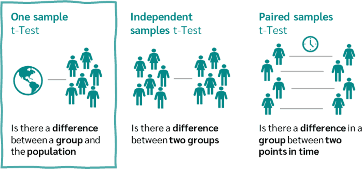
One-Sample T-Test: Compares the mean of a single group to a known value or standard.
Two-Sample T-Test (Independent): Compares the means of two independent groups.
Paired T-Test (Dependent): Compares the means of two related groups or measurements.
One-Tailed vs. Two-Tailed T-Tests

Before getting into the specifics of one-tailed and two-tailed t-tests, lets pause to distinguish these from the previously discussed one-sample, two-sample, and paired t-tests:
Note
difference between “-sampled” and “-tailed” terminology
“One-sample,” “two-sample,” and “paired” refer to the number and nature of the groups being compared.
“One-tailed” and “two-tailed” refer to the directionality of the hypothesis being tested.
Now, let’s explore the differences between one-tailed and two-tailed t-tests:
-
One-Tailed T-Test (or One-Sided T-Test)
A one-tailed t-test is used when the researcher has a specific directional hypothesis about the relationship between the variables being studied.
Key Characteristics:
- Tests for a difference in a specific direction (e.g., greater than or less than).
- The entire significance level (α) is placed in one tail of the distribution.
- Provides more statistical power to detect an effect in the hypothesized direction.
Example: Marine biologists hypothesize that a new conservation method will increase the population of a specific fish species. They would use a one-tailed test to determine if the population after the intervention is significantly greater than before.
Null Hypothesis (H₀): The new conservation method does not increase the fish population. Alternative Hypothesis (H₁): The new conservation method increases the fish population.
When to Use:
- You have strong theoretical or empirical reasons to expect a difference in a specific direction.
- You’re only interested in an effect in one direction and would treat an opposite effect the same as no effect.
-
Two-Tailed T-Test (or Two-Sided T-Test)
A two-tailed t-test is used when the researcher wants to determine if there’s any significant difference between the groups, without specifying the direction of that difference.
Key Characteristics:
- Tests for any difference in means, regardless of direction.
- The significance level (α) is split between both tails of the distribution.
- More conservative than a one-tailed test, as it requires stronger evidence to reject the null hypothesis.
Example: Researchers are comparing the biodiversity of two different coral reef systems but have no prior expectation about which system might have higher biodiversity.
Null Hypothesis (H₀): There is no difference in biodiversity between the two coral reef systems. Alternative Hypothesis (H₁): There is a difference in biodiversity between the two coral reef systems (in either direction).
When to Use:
- You don’t have a specific prediction about the direction of the difference.
- You’re interested in any potential difference, regardless of direction.
- You want to be more conservative in your analysis.
The choice between a one-tailed and two-tailed test is crucial and should be made before data collection, based on the research question and prior knowledge. Incorrectly choosing a one-tailed test when a two-tailed test is appropriate can lead to misleading results and is generally considered poor statistical practice.
In environmental and marine studies, two-tailed tests are often preferred unless there’s a strong theoretical basis for a directional hypothesis. This approach allows researchers to detect unexpected results that might be equally important for understanding complex ecological systems.
Note
summary
One-Tailed T-Test:
Tests for an effect in a specific direction
All significance (α) in one tail of distribution
Used when direction of effect is predicted
Example: Testing if treatment increases fish growth (not if it just changes growth)
Two-Tailed T-Test:
Tests for an effect in either direction
Significance (α) split between both tails
Used when direction of effect is not predicted
Example: Testing if treatment affects fish growth (increase or decrease)