After running a Two-way ANOVA and finding significant differences, we need to figure out where these differences are. That’s where post-hoc tests come in. They help us see the specific group differences in detail.
In our example with factors like Temperature and Nutrient affecting Growth, if we found significant main and interaction effects, post-hoc tests tell us which specific groups are different from each other.
Let’s illustrate these concepts with our simulated growth_data_2.
First, we tested the assumptions (previous section) and fit the ANOVA:
# Fitting the model using growth_data_2anova_model_2<-aov(Growth~Temperature*Nutrient, data =growth_data_2)summary(anova_model_2)
                     Df Sum Sq Mean Sq F value   Pr(>F)
Temperature           1   6054    6054   97.84 2.54e-16 ***
Nutrient              1     88      88    1.43    0.235
Temperature:Nutrient  1   6054    6054   97.84 2.54e-16 ***
Residuals            96   5940      62
---
Signif. codes:  0 '***' 0.001 '**' 0.01 '*' 0.05 '.' 0.1 ' ' 1
We see some significant effects of Temperature, and a significant effect of the interaction of Temperature and Nutrient, so we can proceed with doing a post-hoc test.
Tukey’s Honest Significant Difference (HSD) Test
Just like with one-way ANOVAs, we can use Tukey’s HSD to do the post-hoc test. Tukey’s HSD test is a common choice for comparing all group means against each other while taking into account the multiple comparisons being made.
Comparisons are made among all combinations of Temperature and Nutrient.
a. Low:Poor vs. High:Poor:
Diff: Approximately 0 (7.10e-15)
p adj: 1.00
Interpretation: No significant difference in growth.
b. High:Rich vs. High:Poor:
Diff: 17.44
p adj: 0
Interpretation: Significant difference in growth, with Rich Nutrient level at High Temperature having higher growth.
c. Low:Rich vs. High:Poor:
Diff: -13.68
p adj: Approximately 0 (1e-07)
Interpretation: Significant difference, with Low Temperature and Rich Nutrient having lower growth than High Temperature and Poor Nutrient.
d. High:Rich vs. Low:Poor:
Diff: 17.44
p adj: 0
Interpretation: Significant difference with High Temperature and Rich Nutrient showing higher growth than Low Temperature and Poor Nutrient.
e. Low:Rich vs. Low:Poor:
Diff: -13.68
p adj: Approximately 0 (1e-07)
Interpretation: Significant difference with Low Temperature and Rich Nutrient having lower growth.
f. Low:Rich vs. High:Rich:
Diff: -31.12
p adj: 0
Interpretation: Significant difference, with Low Temperature and Rich Nutrient having substantially lower growth than High Temperature and Rich Nutrient.
To summarize, we have several significant interactions indicating that the effect of one factor depends on the level of the other.
This is really hard to interpret on paper, and this is where those significance letters come in handy.
# A tibble: 4 × 4
  Temperature Nutrient  Mean    SE
  <chr>       <chr>    <dbl> <dbl>
1 High        Poor      23.9  1.55
2 High        Rich      41.4  1.45
3 Low         Poor      23.9  1.55
4 Low         Rich      10.2  1.73
Step 2: Compute Significance Letters with multcompView
library(multcompView)# Run the modelcoral_model<-aov(Growth~Temperature*Nutrient, data =growth_data_2)# Compute the lettersexp_letters<-multcompLetters(post_hoc_result$`Temperature:Nutrient`[, 4])$Letterstukey_result<-data.frame(condition =names(exp_letters), groups =exp_letters)rownames(tukey_result)<-NULLtukey_result
  condition groups
1  Low:Poor      a
2 High:Rich      b
3  Low:Rich      c
4 High:Poor      a
Now, we need to split the “condition” column in tukey_result into “Temperature” and “Nutrient” to match the columns in summary_data.
We can use the separate() function from the tidyr package to split the “condition” column into two new columns, “Temperature” and “Nutrient”:
library(tidyr)# Split the 'condition' column into 'Temperature' and 'Nutrient'tukey_result<-tukey_result%>%separate(condition, into =c("Temperature", "Nutrient"), sep =":")tukey_result
  Temperature Nutrient groups
1         Low     Poor      a
2        High     Rich      b
3         Low     Rich      c
4        High     Poor      a
Now we can combine the groups column from tukey_result with summary_data based on the Temperature and Nutrient columns using the left_join() function from the dplyr package.
# Using left_join to merge datasummary_data<-summary_data%>%left_join(tukey_result, by =c("Temperature", "Nutrient"))summary_data
# A tibble: 4 × 5
Temperature Nutrient Mean SE groups
<chr> <chr> <dbl> <dbl> <chr>
1 High Poor 23.9 1.55 a
2 High Rich 41.4 1.45 b
3 Low Poor 23.9 1.55 a
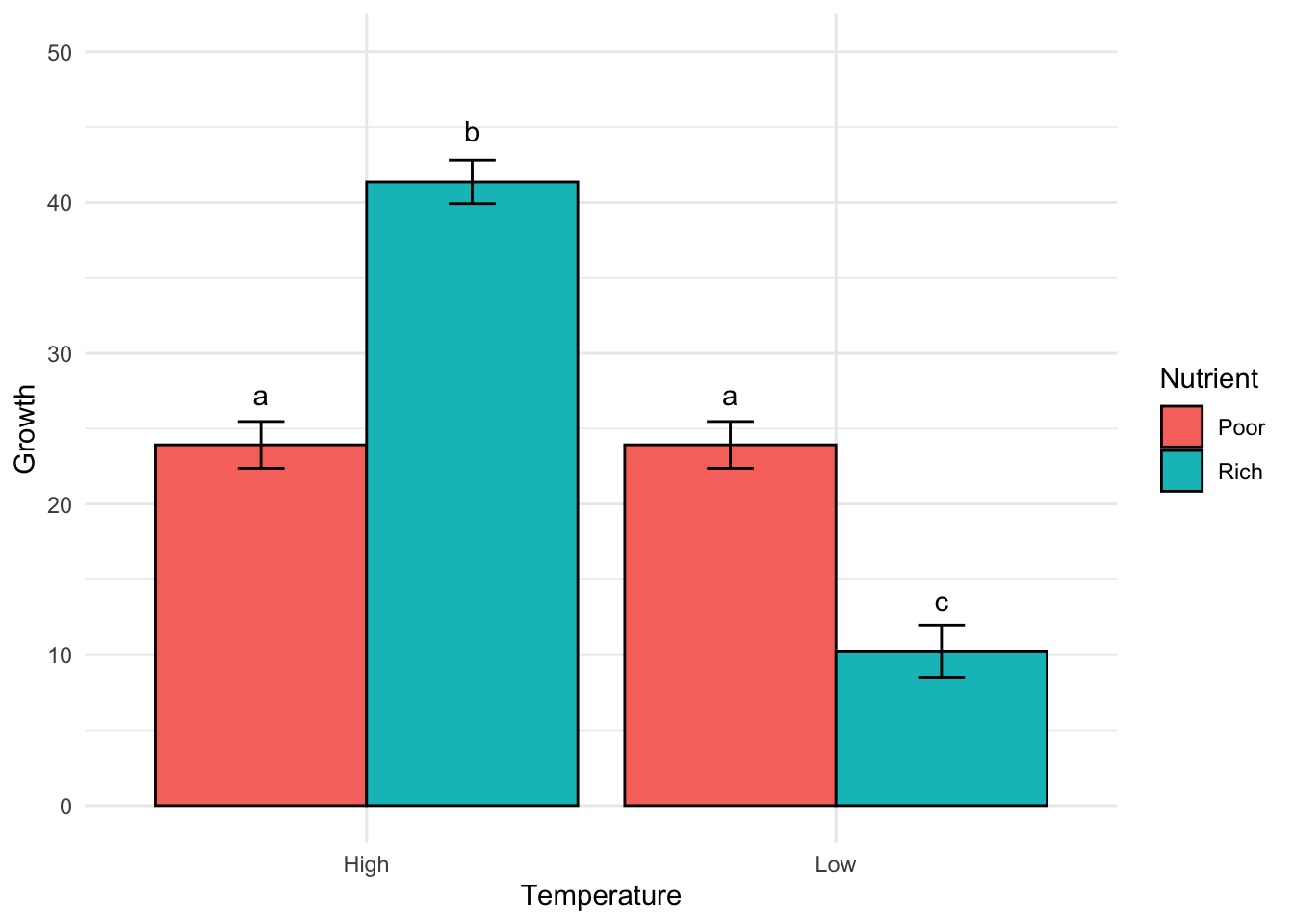
4 Low Rich 10.2 1.73 c
Isn’t this easier to interpret than the Tukey HSD output?
The bar plot clearly shows the significant differences between the groups, with the significance letters indicating which groups are statistically different from each other. We can see that the effect of Temperature on Growth depends on the Nutrient level, with the High Temperature and Rich Nutrient combination having the highest growth, and the Low Temperature and Rich Nutrient combination having the lowest growth.