Mechanics of ANOVA

Partitioning variance

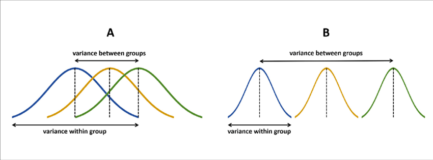
In simple terms, ANOVA works by testing whether between-group variance is greater than what we’d expect by random chance, where this random chance is represented by something called within-group variance.

This involves dividing (or partitioning) the variance into its component parts:

Between-group Variance: This measures the variation in the sample means. In other words, how much do group averages differ from the overall average?
Within-group Variance: This captures the natural variability within each group, i.e., the variation not explained by our grouping factor (like MPA type).

then computing an F-statistic.

\[ F = \frac{\text{Between-group Variance}}{\text{Within-group Variance}} \]

It sounds fancy, but its just the ratio that tells us if the variance between groups is higher than the variance within groups.

A large F-statistic suggests that the differences between group means are more than what we would expect by chance.

ANOVA by hand

Lets pop the hood on ANOVA. Dont worry, there’s a much easier way to do this.

1. Compute the Total Sum of Squares (SST)

This is the variance in the dependent variable without considering the groups.

\[ SST = \sum_{i=1}^{N} (Y_i - \bar{Y})^2 \]

Where:

\(Y_i\) is each individual data point, and \(\bar{Y}\) is the grand mean (the mean of all data points regardless of group).

# Calculate the grand mean
grand_mean <- mean(data_fish_mpa$Fish_Biomass)

# Calculate SST
SST <- sum((data_fish_mpa$Fish_Biomass - grand_mean)^2)
print(SST)

[1] 32939

2. Compute the Between-group Sum of Squares (SSB) This is the variance explained by the groups.

\[ SSB = \sum_{j=1}^{k} n_j (\bar{Y_j} - \bar{Y})^2 \]

Where: \(n_j\) is the number of observations in group \(j\), \(\bar{Y_j}\) is the mean of group \(j\), and \(k\) is the number of groups.

# Calculate SSB
group_means <- tapply(data_fish_mpa$Fish_Biomass, data_fish_mpa$MPA_Type, mean)
group_counts <- table(data_fish_mpa$MPA_Type)
SSB <- sum(group_counts * (group_means - grand_mean)^2)
print(SSB)

[1] 19869

3. Compute the Within-group Sum of Squares (SSW)

This is the variance not explained by the groups.

\[ SSW = SST - SSB \]

# Calculate SSW
SSW <- SST - SSB
print(SSW)

[1] 13070

4. Compute the Mean Squares

Between-group Mean Square (MSB):

This is the variance explained by the groups, adjusted for the number of groups.

\[ MSB = \frac{SSB}{k-1} \]

Within-group Mean Square (MSW):

This is the variance not explained by the groups, adjusted for the number of observations and groups.

\[ MSW = \frac{SSW}{N-k} \]

Where: \(N\) is the total number of observations and \(k\) is the total number of groups

# Calculate Mean Squares
k <- length(unique(data_fish_mpa$MPA_Type))
N <- nrow(data_fish_mpa)

MSB <- SSB / (k - 1) # divided by Between-group degrees of freedom
MSW <- SSW / (N - k) # divided by within-group degrees of freedom

print(MSB)

[1] 9934.5

print(MSW)

[1] 88.908

5. Compute the \(F\) Statistic

As we previously discussed: \[ F = \frac{MSB}{MSW} \]

Remember, a higher F-statistic suggests that the differences between group means are more than what we would expect by chance.

# Calculate F statistic
F_statistic <- MSB / MSW

# Print the F statistic
F_statistic

[1] 111.74

Ok, we know practically that this value means the ratio of between group variance to within group variance. But how do we know if this is significant? This is where critical values come in.

6. Critical Value and p-value: We need to find the critical value needed to reject the null hypothesis and the p-value. The critical value is the value that the F-statistic must exceed to be significant at a given significance level, or alpha (here, and almost always, our alpha is 0.05).

To find the critical value for a given alpha level (e.g., 0.05 for 95% confidence), you use the qf() function. To find the p-value for the computed \(F\) statistic, you use the pf() function. We previously used a similar function to compute a t-test the long way, but we used qt() function instead.

Here we are finding the critical value for the F-distribution with \(k-1\) and \(N-k\) degrees of freedom.

alpha <- 0.05
df1 <- k - 1 # Between-group degrees of freedom
df2 <- N - k # Within-group degrees of freedom

critical_value <- qf(1 - alpha, df1, df2)

p_value <- 1 - pf(F_statistic, df1, df2)
print(p_value)

[1] 0

The p-value gives the probability of observing a value as extreme as, or more extreme than, the observed \(F\) statistic, given that the null hypothesis is true.

Our p-value is very small (showing zero here but this may look more like a e-16 in the anova output), so we reject our null hypothesis.

Comparing long hand to `aov()`

That was a lot of work to get to p = 0, and we get a similar result when we run the aov() function.

summary(aov(Fish_Biomass ~ MPA_Type, data = data_fish_mpa))

             Df Sum Sq Mean Sq F value Pr(>F)    
MPA_Type      2  19869    9935     112 <2e-16 ***
Residuals   147  13070      89                   
---
Signif. codes:  0 '***' 0.001 '**' 0.01 '*' 0.05 '.' 0.1 ' ' 1

compare the outputs from this table to what we calculated above!

Partitioning variance

ANOVA by hand

Comparing long hand to aov()

Comparing long hand to `aov()`