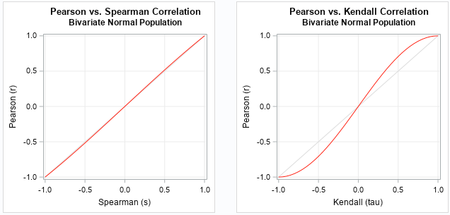
Relationships between Pearson, Spearman, and Kendall Correlation in a bivariate normal population (source)
Types of Correlation Measures
Pearson’s Correlation Coefficient
Pearson’s correlation quantifies the linear relationship between two continuous variables. It’s calculated as the covariance of the two variables divided by the product of their standard deviations:
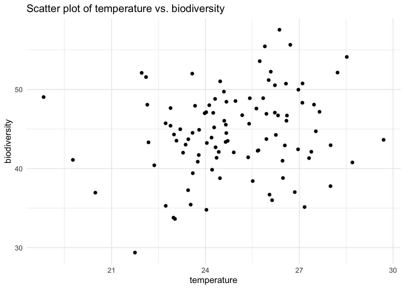
measures the linear relationship between two variables. It assumes that the relationship is linear and sensitive to the actual values of the data. In this case, the relationship between temperature and biodiversity may not be perfectly linear, which is why the correlation is moderate rather than stronger.
Spearman’s correlation (0.176):
measures the rank-based relationship between two variables, meaning it looks at the monotonicity of the relationship. This method is less sensitive to outliers and assumes a monotonic relationship (either increasing or decreasing). Since it doesn’t assume linearity, the lower value compared to Pearson might indicate that while temperature and biodiversity have some association, it may not be strictly monotonic, or there may be variability in the rankings.
Kendall’s Tau (0.125):
Kendall’s Tau also measures the rank-based relationship but is typically more conservative than Spearman’s. It looks at the concordance between pairs of data points (how often the ranks of the two variables agree). This metric tends to be lower because it’s a stricter assessment of monotonicity. The lower value suggests that there is even less agreement in the rank-order between temperature and biodiversity compared to Spearman’s.
Important
A relationship between two variables is monotonic if, as one variable increases (or decreases), the other variable consistently moves in one direction—either always increasing or always decreasing.
Choosing the Right Measure
1. Visual Inspection
Start with a scatter plot:
ggplot(ecosystem_data, aes(x=temperature, y=biodiversity))+geom_point()+# geom_smooth(method="lm", col="red") +theme_minimal()+labs(title="Scatter plot of temperature vs. biodiversity")
2. Check for Linearity
Assess if the relationship appears linear. Non-linear patterns may require Spearman’s or Kendall’s methods.
    Shapiro-Wilk normality test

data:  ecosystem_data$biodiversity
W = 0.99392, p-value = 0.9369
4. Consider Sample Size and Ties
For small samples (n < 30) or data with many ties, Kendall’s Tau may be more appropriate than Spearman’s.
In this context, ties are instances where two or more observations have the same value.
5. Interpretability
Pearson’s r^2 represents the proportion of variance in one variable explained by the other. Spearman’s ρ^2 represents the proportion of variance in ranks explained. Kendall’s τ represents the probability of concordance minus the probability of discordance.
Additional Considerations
Bootstrapping for Confidence Intervals
Bootstrapping is a resampling technique that can provide more robust estimates of correlation coefficients (or anything that you want to measure). It involves repeatedly sampling with replacement from the dataset to calculate confidence intervals.
For more robust estimates, consider bootstrapping to calculate confidence intervals:
library(boot)# Function to compute correlationcor_func<-function(data, indices){d<-data[indices,]return(cor(d$temperature, d$biodiversity, method="pearson"))}# Bootstrappingset.seed(123)boot_results<-boot(ecosystem_data, cor_func, R=1000)# Print resultsprint(boot.ci(boot_results, type="bca"))
BOOTSTRAP CONFIDENCE INTERVAL CALCULATIONS
Based on 1000 bootstrap replicates

CALL :
boot.ci(boot.out = boot_results, type = "bca")

Intervals :
Level       BCa
95%   ( 0.0003,  0.3971 )
Calculations and Intervals on Original Scale
Partial Correlation
When you want to measure the relationship between two variables while controlling for the effect of one or more other variables, use partial correlation:
   estimate    p.value statistic   n gp  Method
1 0.1875848 0.06298709  1.880885 100  1 pearson
This partial correlation shows the relationship between temperature and biodiversity, controlling for the effect of salinity.
The choice of correlation measure should be guided by your data’s characteristics, research question, and the assumptions you can reasonably make. Each method offers unique insights, and sometimes using multiple methods can provide a more comprehensive understanding of your data.