ANCOVA Tutorial: Shark Swimming

Research Context

During a comparative study of swimming speeds between two shark species, researchers encountered unexpectedly high variability in their measurements. Initial analysis using a simple one-way ANOVA revealed no significant differences between species (p > 0.05). However, closer examination of the data suggested that water temperature, which varied naturally during the study period (20-28°C), might be systematically affecting swimming speeds.

This situation presented a classic case for Analysis of Covariance (ANCOVA). While ANOVA could test for species differences, it couldn’t account for the continuous variable (temperature) that appeared to influence the dependent variable (swimming speed). ANCOVA extends the ANOVA framework by incorporating this type of continuous predictor, known as a covariate, allowing researchers to:

Control for the effect of temperature on swimming speed
Test for species differences after adjusting for temperature effects
Examine whether temperature affects species differently

Data and Initial Exploration

(simulating some data…..)

# Set seed for reproducibility
set.seed(789)

# Create sample data
n_per_group <- 40

# Generate temperatures that span the same range for both species
temps <- runif(n_per_group, 20, 28)  # Temperature range 20-28°C

shark_data <- data.frame(
  species = factor(rep(c("Mako", "White tip"), each = n_per_group)),
  temp = c(temps, temps),  # Same temperature range for both species
  length = rnorm(n_per_group * 2, 200, 10)  # Control for length
)

# Generate swimming speeds where:
# - Temperature has a strong positive effect
# - Species A is actually faster when controlling for temperature
shark_data$speed <- with(shark_data, 
                        3 * temp +                     # strong temperature effect
                        ifelse(species == "Mako", 2, 0) + # Species A is faster at same temp
                        rnorm(n_per_group * 2, 0, 2))    # random noise

In this dataset, each row represents an individual shark observation, including the species (categorized as either mako or white tip), the water temperature in degrees Celsius at the time of observation, the shark’s body length in centimeters, and its swimming speed in meters per second.

The analysis framework consists of three key variables. The independent variable is species, a categorical factor with two levels (mako and white tip). Swimming speed serves as the dependent variable, measured as a continuous value in meters per second. Water temperature acts as a covariate in the analysis, providing continuous measurements in degrees Celsius that might influence swimming speed independently of species differences.

The researchers formulated their hypotheses to test for species differences while accounting for temperature effects. Regarding their main effects, their null hypothesis (H₀) states that no difference exists in swimming speeds between species after controlling for temperature. their main effect alternative hypothesis (H₁) is that there is a true difference in swimming speeds exists between species when temperature is taken into account.

Initial Visual Assessment

First, let’s examine the raw speed differences between species:

library(ggplot2)

ggplot(shark_data, aes(x = species, y = speed)) +
  geom_boxplot(fill = "lightblue") +
  theme_bw() +
  labs(title = "Raw Swimming Speed Comparison Between Species",
       x = "Species",
       y = "Swimming Speed (m/s)")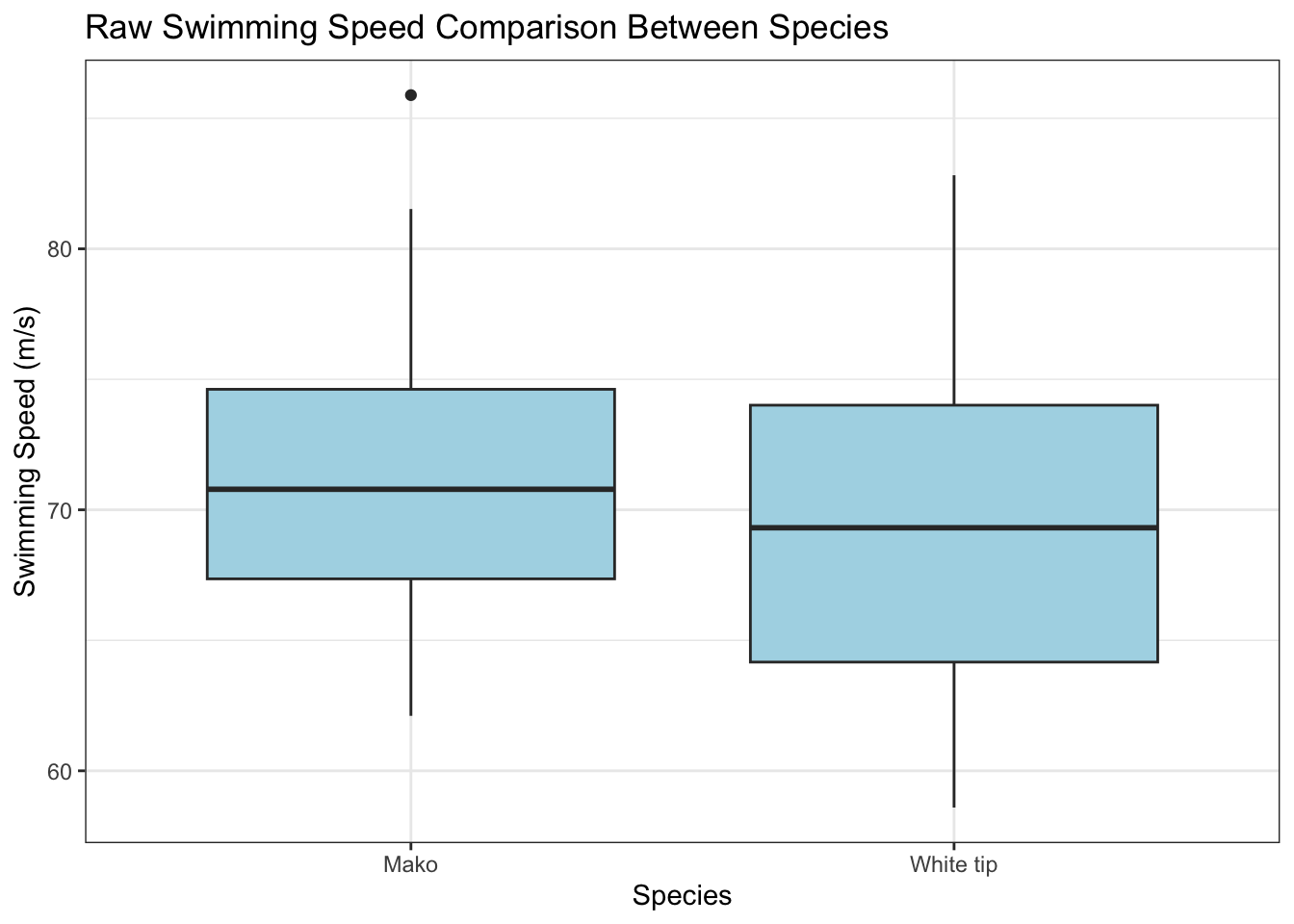

The boxplot suggests similar swimming speeds between species. However, let’s examine how temperature might influence these speeds:

ggplot(shark_data, aes(x = temp, y = speed, color = species)) +
  geom_point(alpha = 0.6) +
  geom_smooth(method = "lm", se = FALSE) +
  theme_bw() +
  labs(title = "Swimming Speed vs Temperature by Species",
       x = "Temperature (°C)",
       y = "Swimming Speed (m/s)")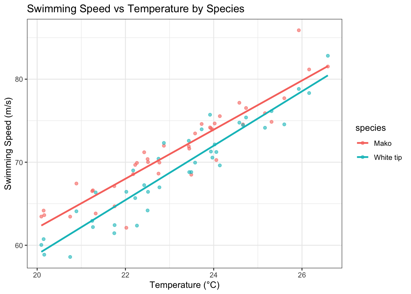

Testing ANCOVA Assumptions

Before proceeding with ANCOVA, we must verify several key assumptions:

1. Homogeneity of Regression Slopes

# Test for interaction between species and temperature
interaction_model <- aov(speed ~ species * temp, data = shark_data)
summary(interaction_model)

             Df Sum Sq Mean Sq F value   Pr(>F)    
species       1   98.0    98.0  22.738 8.76e-06 ***
temp          1 2202.9  2202.9 511.023  < 2e-16 ***
species:temp  1    5.6     5.6   1.308    0.256    
Residuals    76  327.6     4.3                     
---
Signif. codes:  0 '***' 0.001 '**' 0.01 '*' 0.05 '.' 0.1 ' ' 1

The non-significant interaction term suggests parallel slopes, meeting this assumption.

2. Normality of Residuals

# Fit the ANCOVA model
ancova_model <- aov(speed ~ species + temp, data = shark_data)

# Check residuals
hist(rstandard(ancova_model), 
     main = "Histogram of Residuals",
     xlab = "Residuals")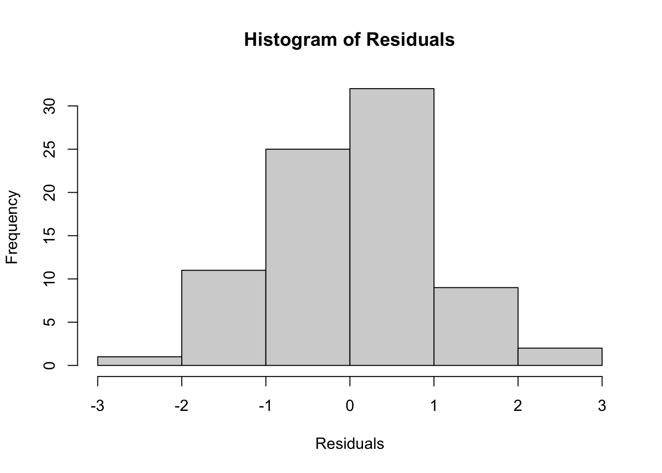

shapiro.test(rstandard(ancova_model))


    Shapiro-Wilk normality test

data:  rstandard(ancova_model)
W = 0.99104, p-value = 0.8568

The residuals appear approximately normally distributed.

3. Homogeneity of Variances

plot(ancova_model, 1)  # Residuals vs Fitted plot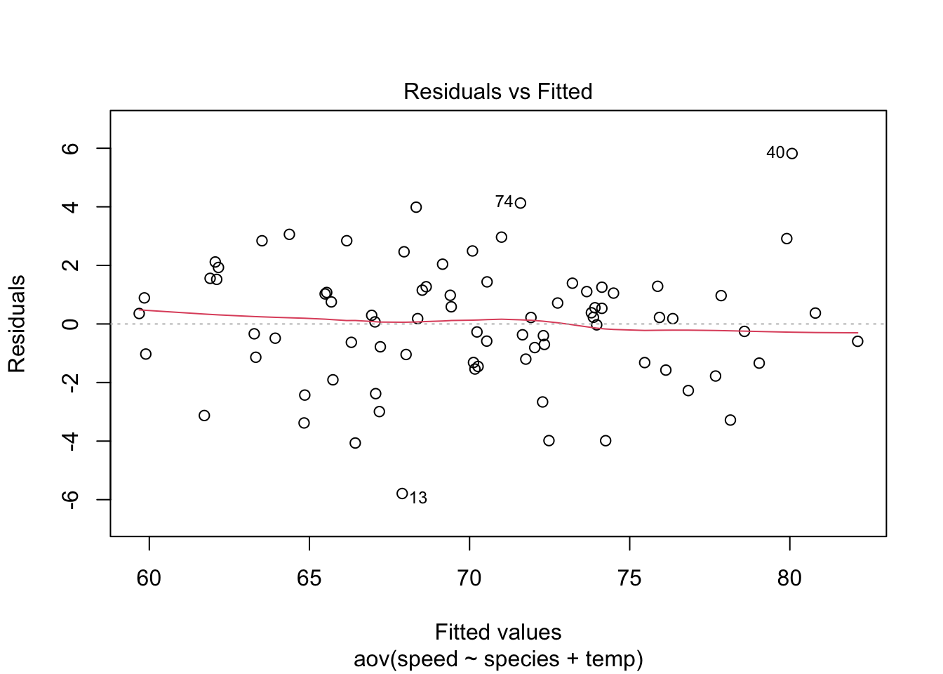

bartlett.test(speed ~ species, data = shark_data)


    Bartlett test of homogeneity of variances

data:  speed by species
Bartlett's K-squared = 0.29373, df = 1, p-value = 0.5878

Comparing Models: ANOVA vs. ANCOVA

Let’s compare the results of a simple ANOVA with our ANCOVA:

# Simple ANOVA
simple_model <- aov(speed ~ species, data = shark_data)
cat("ANOVA Results:\n")

ANOVA Results:

summary(simple_model)

            Df Sum Sq Mean Sq F value Pr(>F)  
species      1     98   98.02   3.015 0.0865 .
Residuals   78   2536   32.52                 
---
Signif. codes:  0 '***' 0.001 '**' 0.01 '*' 0.05 '.' 0.1 ' ' 1

cat("\nANCOVA Results:\n")


ANCOVA Results:

summary(ancova_model)

            Df Sum Sq Mean Sq F value   Pr(>F)    
species      1   98.0    98.0   22.65 8.93e-06 ***
temp         1 2202.9  2202.9  508.99  < 2e-16 ***
Residuals   77  333.3     4.3                     
---
Signif. codes:  0 '***' 0.001 '**' 0.01 '*' 0.05 '.' 0.1 ' ' 1

The comparison between ANOVA and ANCOVA results reveals how critical it was to account for temperature in this analysis. The initial ANOVA suggested non-significant differences between species (F[1,78] = 3.015, p = 0.0865), which might have led researchers to conclude that the species showed similar swimming speeds. This model left most of the variation unexplained, with substantial residual variance (Mean Sq = 32.52).

However, the ANCOVA tells a markedly different story. After accounting for temperature, clear species differences emerged (F[1,77] = 22.65, p = 8.93e-06). Temperature itself proved to be a powerful predictor of swimming speed (F[1,77]= 508.99, p < 2e-16), suggesting it’s a crucial factor in shark movement behavior. Most notably, incorporating temperature as a covariate dramatically reduced the residual variance from 27.34 to just 4.3, indicating that much of the “noise” in the original analysis was actually attributable to temperature effects.

The stark contrast between these results demonstrates why accounting for temperature was essential. What initially appeared to be random variation in swimming speeds was largely explained by temperature differences. By controlling for this environmental factor, the ANCOVA revealed genuine species differences that were previously masked by temperature effects.

Let’s examine the model fit improvements:

cat("ANOVA R-squared and RSE:\n")

ANOVA R-squared and RSE:

summary.lm(simple_model)$r.squared

[1] 0.03721062

summary.lm(simple_model)$sigma

[1] 5.7022

cat("\nANCOVA R-squared and RSE:\n")


ANCOVA R-squared and RSE:

summary.lm(ancova_model)$r.squared

[1] 0.8734877

summary.lm(ancova_model)$sigma

[1] 2.080392

The dramatic improvement in model fit statistics further emphasizes the importance of including temperature in our analysis. The initial ANOVA model explained only about 3.7% of the variation in swimming speeds (R² = 0.037), leaving most of the behavioral differences unexplained. This model also showed high residual standard error (RSE = 5.7 m/s), indicating poor prediction accuracy.

In contrast, the ANCOVA model, which accounts for temperature, explains approximately 87% of the variation in swimming speeds (R² = 0.873). This improvement in explanatory power suggests that temperature and species together account for the vast majority of variation in shark swimming behavior. The residual standard error was also reduced by more than half (RSE = 2.08 m/s), indicating much more precise estimates of swimming speed.

These model fit statistics tell us two important things: first, that temperature is a crucial predictor of swimming speed, explaining a large portion of the variation that was previously considered random noise. Second, that only by accounting for temperature could we accurately detect and measure the true differences between species. This highlights why researchers must carefully consider environmental variables when studying behavioral differences - failing to account for such variables can mask important biological patterns and lead to incorrect conclusions about species differences.

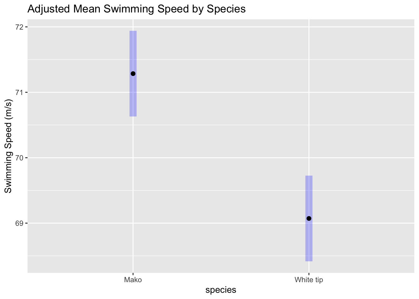
We can also visualize the adjusted means to better understand species differences. emmeans, a package for estimated marginal means, can help calculate and plot the means. The means are adjusted by the covariate to provide a clearer picture.

# Calculate adjusted means
library(emmeans)
adjusted_means <- emmeans(ancova_model, "species")
plot(adjusted_means) +
  labs(title = "Adjusted Mean Swimming Speed by Species",
       x = "Swimming Speed (m/s)") +
  coord_flip()