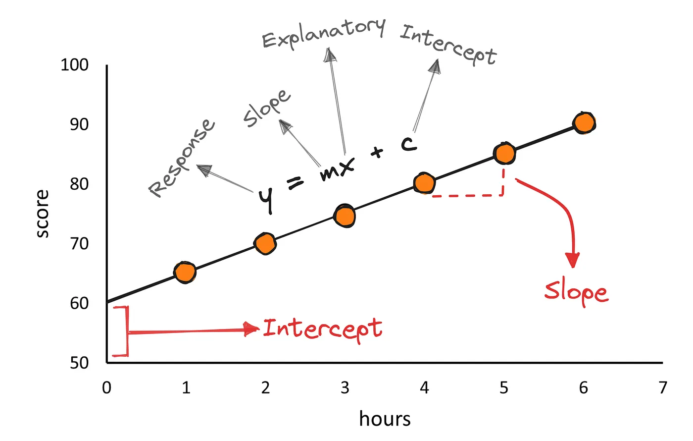
At its core, linear regression is about finding the best line that fits a set of data points. Imagine plotting data on a graph and then drawing a straight line that best captures the trend in that data. This line can then be used to make predictions. In mathematical terms, this line is represented by the equation:
\[ Y=β_0+β_1X+ϵ \]
Where:
\(Y\) is the dependent variable (what we’re trying to predict),
\(X\) is the independent variable (the input),
\(β_0\) is the y-intercept,
\(β_1\) is the slope of the line, and
\(ϵ\) represents the residuals or errors (the difference between observed and predicted values).
The term “linear” in linear regression refers to the linearity of the relationship between the dependent and independent variables. This means that the relationship can be represented by a straight line. This simplicity allows for clear interpretations and is especially useful when starting with data analysis.
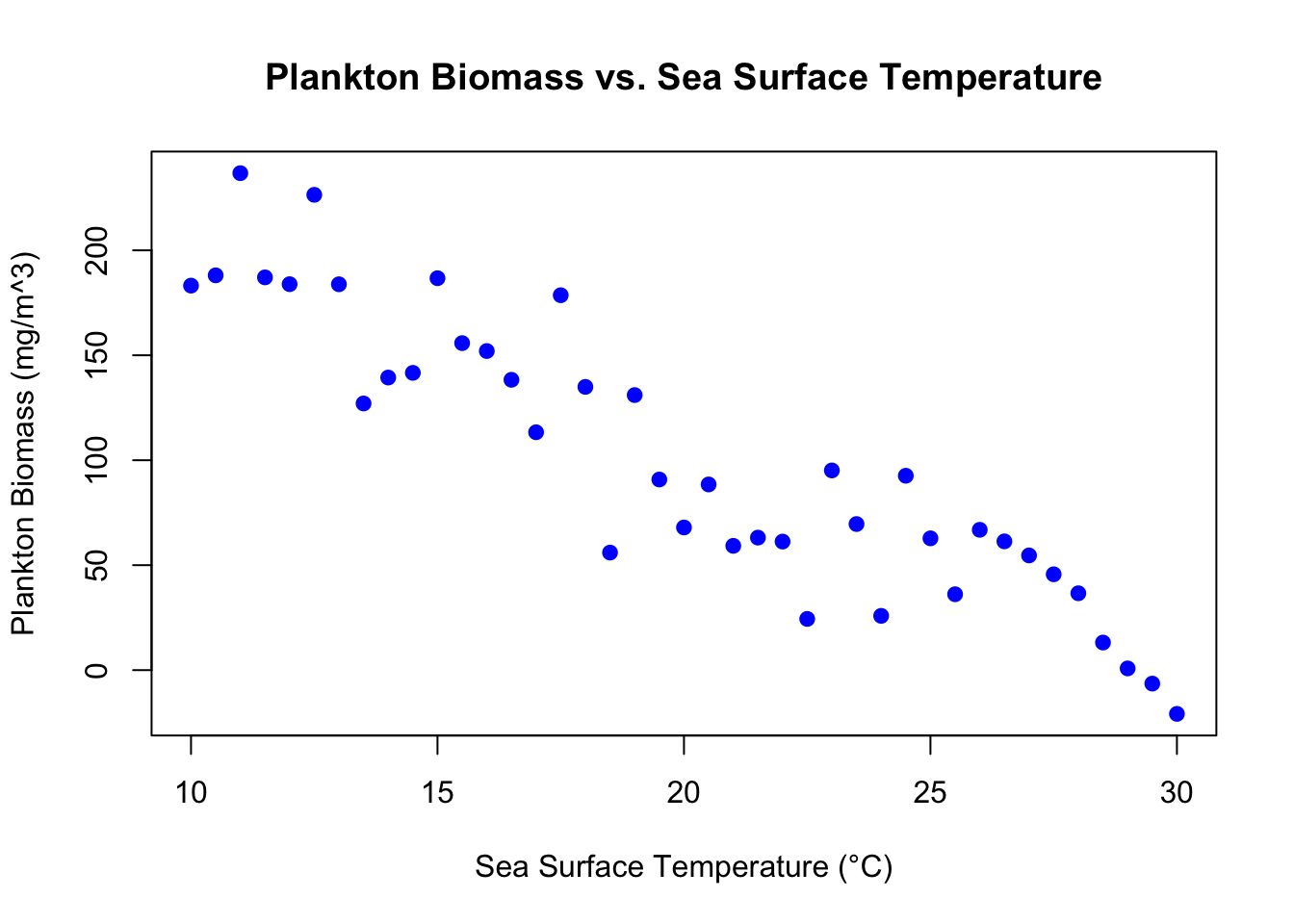
Marine environments are full of variables that have potential linear relationships. Understanding the relationship between sea surface temperature and coral bleaching, or between nutrient levels and algal blooms, can be pivotal in marine conservation and management.
Example Data: Sea Surface Temperature (SST) vs. Plankton Biomass
For our example, let’s consider some (made up) monthly averaged data of sea surface temperature (in °C) and the corresponding plankton biomass (in mg/m^3) for a specific coastal region.
# Hypothetical Dataset.seed(123)# Setting seed for reproducibilitySST<-seq(10, 30, by=0.5)# Temperature from 10°C to 30°Cplankton_biomass<-300-10*SST+rnorm(length(SST), mean=0, sd=30)# Linear relationship with added noise# Combining data into a data frameplankton_temp_data<-data.frame(SST, plankton_biomass)# Visualizing the dataplot(plankton_temp_data$SST, plankton_temp_data$plankton_biomass, xlab="Sea Surface Temperature (°C)", ylab="Plankton Biomass (mg/m^3)", main="Plankton Biomass vs. Sea Surface Temperature", pch=19, col="blue")
think about it: as sea surface temperature increases, what happens to plankton biomass?
to test this relationship statistically, we use linear regression.
Here is the R code to make the linear regression model
model<-lm(plankton_biomass~SST, data =plankton_temp_data)
plankton_biomass ~ SST specifies the formula for the linear regression. Here, we are predicting plankton_biomass as a function of SST (Sea Surface Temperature). plankton_biomass is the dependent variable (or response), and SST is the independent variable (or predictor).
data = plankton_temp_data tells R to use the data frame plankton_temp_data for this analysis. Within this data frame, there should be columns named plankton_biomass and SST.
The result of this function is an object (in this case named model) that contains all the information about the linear regression, including coefficients, residuals, and other diagnostic measures.
This model does the fitting of the line for you, and tells you if the best fit line has a slope and intercept that are significantly different from zero.
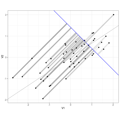
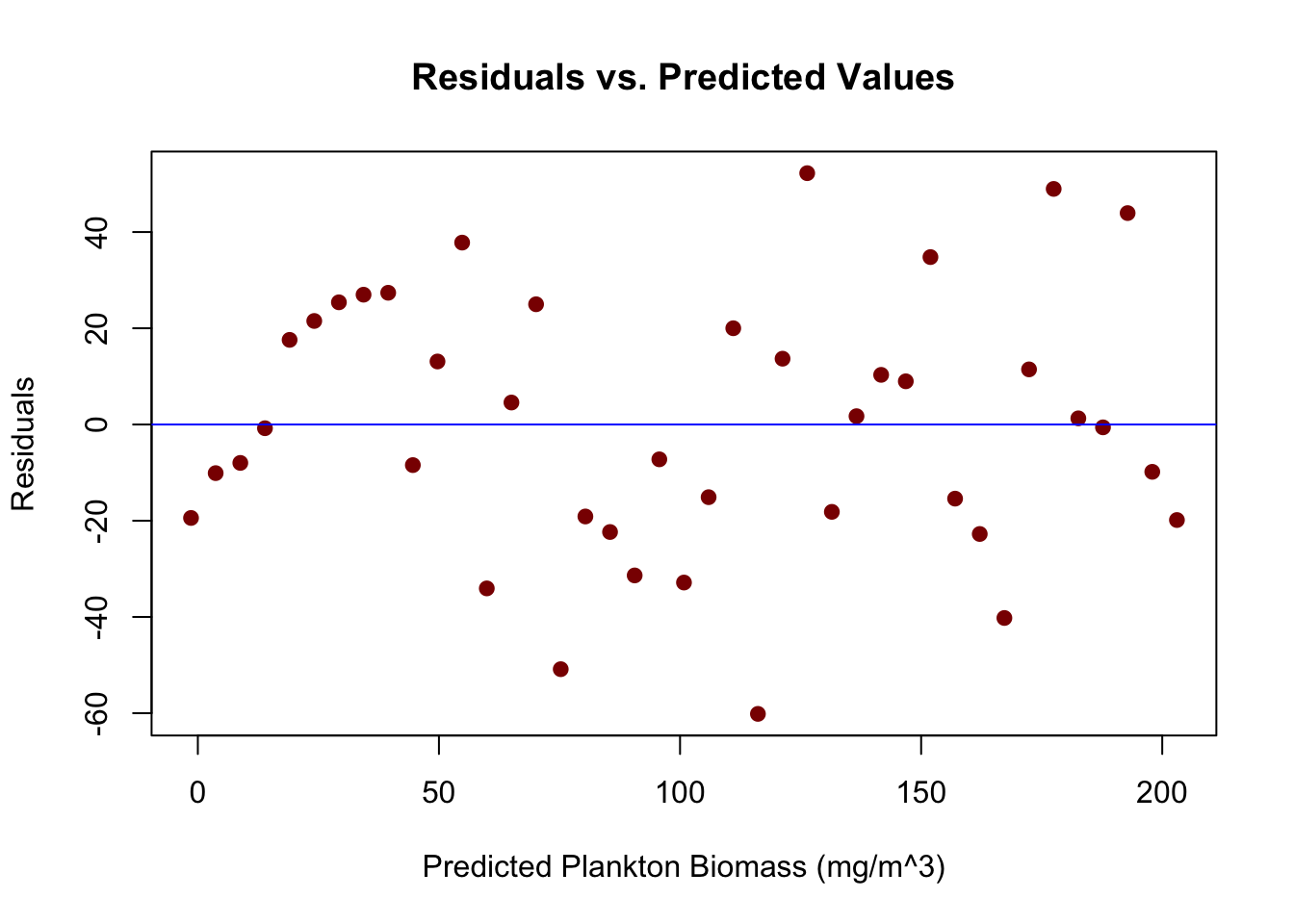
Think about it as if each point is connected to the line via a rubber band. The line of best fit (the regression line) is the one that snaps to minimize stretch on any single rubber band. The residuals are the distances between each point and the line, and the sum of squared error tells you as a whole how far that line is from the data. Lets extract and view our residuals and SSE from model below.
Now, let’s visualize the residuals to understand the spread and pattern:
predicted_values<-fitted(model)plot(predicted_values, residuals_data, xlab="Predicted Plankton Biomass (mg/m^3)", ylab="Residuals", main="Residuals vs. Predicted Values", pch=19, col="darkred")abline(h=0, col="blue")# adds a horizontal line at y=0